An introduction to mathematical modeling in systems biology
Welcome the lab, down below you can find an illustration of how you will work through the lab. You will be introduced to some hypotheses of a biological system and formulate models of these to describe some experimental data. You will test the different hypothesis to see if you can reject any of them using experimental data and making predictions with the models.
Modelling cycle.
Introduction
First thing to do, is to read the introduction "hidden" below.
Click to expand introduction
This is a new version of the lab introduced in 2019, more oriented towards writing your own scripts to further your understanding of the different parts, and also to give you valuable programming skills for your future career. The current version of the lab is implemented in MATLAB, but you are free to pick other languages if you can find the proper tools. Please note that the supervisors will only help with code issues in MATLAB.
Purpose of the lab
This lab will on a conceptual level guide you through all the main sub-tasks in a systems biology project: model formulation, optimization of the model parameters with respect to experimental data, model evaluation, statistical testing, (uniqueness) analysis, identification of interesting predictions, and testing of those predictions.
How to pass
To pass the entire lab you need to individually pass the quiz on LISAM ("Computer lab - coding version" if you're doing this version). Along the instructions, there are check-points that correspond to questions in the quiz. These are marked with checkpoint x.
The deadline to be approved is at the final computer lab session
Preparations
Get familiar with MATLAB by doing Mathworks intro tutorial. You can find the tutorial at this link.
Most of the tasks below start with Background. If one wants to prepare, these can be read in advance of the lab. They are written more as a background about the different topics, and can be read without solving the previous tasks.
Getting MATLAB running
Follow the installation guide on Lisam, or here.
In the computer halls
If you are working on a Linux based computer in the computer hall, use the following steps to get MATLAB going.
First, open a terminal. Then run module add prog/matlab/9.5.
Note that the version sometimes changes, if 9.5 can't be found, check available versions with module avail.
ThinLinc (from home)
If you are working from the computer hall you can access your files from home using ThinLinc. To get started, firstly download the ThinLinc client for your operative system from Cendio.
Login to ThinLinc requires two-step verification, for more information and instructions to activate two-step verification see the infomration from Liu.
You sign in to the server thinlinc.edu.liu.se using the same username and password as you would sign in to a computer in the computer halls. When signed in, you can run MATLAB using the module add prog/matlab/9.5 command in a terminal.
Interpreting function relationship graphs
Throughout this lab, we will use graphs similar to the one below to illustrate how different functions communicate.
Here, a function F1 is sending two arguments, arg1, arg2, to another function F2. F2 then returns arg3to function F1.
Questions?
If you have questions when going through the lab, first have a look at Q&A in the course room (LISAM), if you cannot find an answer, bring the questions to the computer lab sessions, or you can also raise them in Teams. In many situations, your fellow students probably know the answer to your question. Please help each other if possible!
Main computer lab tasks
Implementing and simulating a model
Background
Now, let us start with implementing a simple model! Here we will learn the basics of how to create models and simulate them. Implement a model with a single state A, with a constant increase () and an initial amount of 4 (). Let the amount of be the measurement equations ().
Software/toolboxes/compilers
Note: do not work from a cloud synced folder (such as a OneDrive folder).
This has repeatedly been observed to cause unknown issues and give performance degradation.
C-compiler
First check if you have the compilers installed and working in MATLAB. In the MATLAB command window run mex -setup. If Matlab doesn't find a compiler, install one (e.g. mingw). Instructions for installation should appear when running mex -setup if no compiler is found.
Simulation toolbox (IQM tools)
Then, download IQM toolbox from LISAM or here, extract the files, move to the folder in MATLAB and then run the file called installIQMtoolsInitial.m. This will compile the simulation toolbox and make it usable in MATLAB. The next time you start MATLAB, you do not have to compile the toolbox, but you will need to install the toolbox again. In subsequent starts, run installIQMtools.m. Now, move back to the folder where you will work on this lab.
Optimization toolbox
Later in the lab, we will optimize the parameter values of the models using the MEIGO toolbox. This toolbox is also available on LISAM and here. Again, extract the files and make it usable by running install_MEIGO.m from the extracted MEIGO folder. In subsequent starts of MATLAB, you will need to run the install_MEIGO.m tools.
Now that all toolboxes have been installed, you will continue with creating a first simple model to test the simulation toolbox.
Templates
To help you with getting started, we have created some templates for the scripts you will create. They are available here. These templates are fully optional. Download and extract the files to your working directory.
File structure
Assuming you have installed all toolboxes and downloaded the templates, your file structure should look like this:
📂computer-exercise
 ┣ 📂IQMtools_V1222_updated
 ┃ ┣ 📂IQMlite
 ┃ ┣ 📂IQMpro
 ┃ ┣ 📜installation.txt
 ┃ ┣ 📜installIQMtools.m
 ┃ ┗ 📜installIQMtoolsInitial.m
 ┣ 📂MEIGO
 ┃ ┣ 📂eSS
 ┃ ┣ 📂examples
 ┃ ┣ 📂VNS
 ┃ ┣ 📜gpl-3.0.txt
 ┃ ┣ 📜install_MEIGO.m
 ┃ ┗ 📜MEIGO.m
 ┣ 📜CostFunction.m
 ┣ 📜Main.m
 ┣ 📜PlotExperiment.m
 ┗ 📜SimulateExperiment.m
Do not put your working files inside the IQMtools or MEIGO folder
Implement a simple model
Create a text file and use the following model formulation. Save it as SimpleModel.txt.
Note that the text file must contain all headers (beginning with “********** “)
********** MODEL NAME
SimpleModel
********** MODEL NOTES
********** MODEL STATES
d/dt(A)=v1
A(0)=4
********** MODEL PARAMETERS
k1=2
********** MODEL VARIABLES
ySim=A
********** MODEL REACTIONS
v1=k1
********** MODEL FUNCTIONS
********** MODEL EVENTS
********** MODEL MATLAB FUNCTIONS
Compile the model
Now, we will first convert your equations into a model object, so that you can then compile the model into a MEX-file. The MEX-file is essentially a way to run C-code inside MATLAB, which is much faster than ordinary MATLAB code.
modelName='SimpleModel'
model=IQMmodel([modelName '.txt']);
IQMmakeMEXmodel(model) %this creates a MEX file which is ~100 times faster
Note: The compiled file will have a filename based on what is written under
****** MODEL NAME, and an ending based on what OS it is compiled on. In this case, SimpleModel.mex[w64/maci64/a64]
Simulate the model
Simulating the model
We will now construct two scripts, a main script that will call your other scripts and a SimulateExperiment script that will do the simulation of the model.
Create a main script
This is the script we will use to call the other functions we create. Here, we will name this script Main. To create a function/script, press “new” in the toolbar and choose function/script.
Create a simulation function (SimulateExperiment)
This simulation function should take (params, modelName, and time) as inputs and returns vectors ySim and timeSim as output. To do this, use the template or click on New in MATLAB's command window and select Function. Edit the input and outputs to use the following structure:
The blue boxes represent a function/script with the name written in it. The black arrows represent the direction a set of arguments is sent between two functions. In the above example, the script Main passes the arguments params, modelName, time to the function SimulateExperiment, that returns ySim back to Main.
In the next step you will implement the actual simulation, but for now, just set ySim to some arbitrary placeholder value and leave the rest of the script empty.
Implement the simulation
Since we have compiled the model, we can now simulate the model by directly calling the MEX file. In practice, we convert the name of the model in the form of a string (in modelName) into a callable function using str2func. In the case of the simple model, the function call would look like this:
% Assumes modelName = 'SimpleModel'
model = str2func(modelName); % Defines a callable function from the string value in modelName
sim = model(time, IC, params); % Simulate the model
Here, sim is the resulting simulation, SimpleModel is the name of the model given when you compiled the model, time are the desired time points to simulate, IC is the initial conditions, and params are the values of the parameter in the model.
Note: it is also possible to skip IC and/or params as inputs. The model will then instead use the values written in the model file (when the MEX-file was compiled). In practice, this is done by passing along [] instead of e.g. IC.
Extra: There exist at least three other (typically less practical) alternative ways to simulate the model:
Three examples are given below:
(Note, IC is the initial conditions)
sim = IQMPsimulate(model, time, IC, paramNames, params)sim = IQMPsimulate(modelName, time, IC, paramNames, params)sim = NameOfTheCompiledModel(time, IC, params)
Alternative 1) takes an IQM model as first input, and will automatically compile the model. This might sound good, but will result in the model being compiled every time a simulation is done. Running a compiled model is much faster, but the compilation takes some time. Therefore, this is a bad idea.
Both alternative 2) and 3) both uses the MEX-compiled model, however 3) uses the file directly and is almost always the best alternative (5x faster and more convenient). This is the method that is used in the example above, we just use the str2func function to convert the string in the modelName variable into a callable funcition.
Using alternative 2), it is possible to only specify custom values of some parameters. The parameters to change is then specified in the paramNames argument. The other parameters will use the model values as defined in the model file during compilation.
In most cases alternative 3) is the best.
Extract the output of simulation
The simulation returns a struct, with many relevant fields. In our case, we are interested in the variable values. You can access these values in the following way:
ySim = sim.variablevalues(:,1);
In this case, we are interested in extracting all values of the first variable.
Make sure to remove the placeholder value.
Dealing with problematic simulations
Sometimes the simulation crashes for certain sets of parameters, and this is fine. However, it can become issues in the scripts. To bypass issues related to crashed simulation, add a try-catch block in your simulation script and return a vector of the same size as ySim should be (the size of time), but with a very large value for each element.
try
    sim = model(time, [], params); % Replace [] with IC to use custom values
    ySim = sim.variablevalues;
    simTime = sim.time;
catch error
    disp(getReport(error)) %Prints the error message.
    ySim=1e20*ones(size(time)); % return some large value
    simTime = time;
end
Note: If you get errors other than CV_ERR_FAILURE, you have another issue than problematic parameter values. Also note that you can disable the printout of the error by commenting out % disp(getReport(error)) if you get too many CV_ERR_FAILURE failure
Now it is time to call your new SimulateExperiment function from your Main script with relevant inputs. For now, set params = 2 (same values as in the model file).
Run Main script
Now, update your Main script to use your SimulateExperiment function to get the simulation.
ySim = SimulateExperiment(params, modelName, time)
Now run the Main script to test that everything works. As a time-vector, use time = 0:0.2:2 (from 0 to 2 with step-lenth 0.2) and for params use the default values (params = []). Does your SimulateExperiment return ySim=[4, 4.4, 4.8, 5.2, 5.6, 6, 6.4, 6.8, 7.2, 7.6, 8]?
[ ] Checkpoint 1: Does your simple model behave as you expected?
Data
Background
During the following exercises you will take on the role of a system biologist working in collaboration with an experimental group.
The experimental group is focusing on the cellular response to growth factors, like the epidermal growth factor (EGF), and their role in cancer. The group have a particular interest in the phosphorylation of the receptor tyrosine kinase EGFR in response to EGF and therefore perform an experiment to elucidate the role of EGFR. In the experiment, they stimulate a cancer cell line with EGFR and use an antibody to measure the tyrosine phosphorylation at site 992, which is known to be involved in downstream growth signaling. The data from these experiments show an interesting dynamic behavior with a fast increase in phosphorylation followed by a decrease down to a steady-state level which is higher than before stimulation (Figure 1).
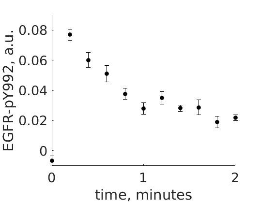
Figure 1: The experimental data. A cancer cell line is stimulated with EGF at time point 0, and the response at EGFR-pY992 is measured
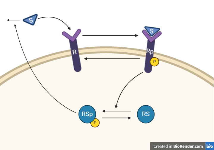
The experimental group does not know the underlying mechanisms that give rise to this dynamic behavior. However, they have two different ideas of possible mechanisms, which we will formulate as hypotheses below. The first idea is that there is a negative feedback transmitted from EGFR to a downstream signaling molecule that is involved in dephosphorylation of EGFR. The second idea is that a downstream signaling molecule is secreted to the surrounding medium and there catalyzes breakdown of EGF, which also would reduce the phosphorylation of EGFR. The experimental group would like to know if any of these ideas agree with their data, and if so, how to design experiments to find out which is the more likely idea.
To generalize this problem, we use the following notation:
EGF – Substrate (S)
EGFR – Receptor (R)
Download and load data
Download the experimental data from here or on LISAM. Place it in your working folder.
Load the experimental data into MATLAB by using the load function in your main script. Remember, you can read more about a function with the command help or doc.
Run your main script and note that the variable is now in the workspace. Click on it and have a look at the subfields. The subfields can be accessed as e.g. expData.time.
Plot data
Create a function that takes data as input and plot all the points, with error bars.
Use the following structure:
Make sure your plots look nice. Give the axes labels.
Useful MATLAB commands:
errorbar, xlabel, ylabel, title, plot
[ ] Checkpoint 2: How does the data look?
Hypotheses
Background
The experimentalists have 2 ideas for how they think the biological system they have studied work. These hypotheses are presented below.
Hypothesis 1

From this knowledge, we can draw an interaction graph, along with a description of the reactions.
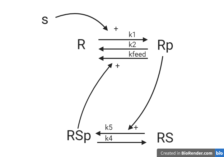
- Reaction 1 is the phosphorylation of the receptor (R). It depends on states R and S with the parameter k1.
- Reaction 2 is the basal dephosphorylation of Rp to R. It depends on the state Rp with the parameter k2.
- Reaction 3 is the feedback-induced dephosphorylation of Rp to R exerted by Rsp. This reaction depends on the states Rp and Rsp with the parameter kfeed.
- Reaction 4 is the basal dephosphorylation of Rsp to RS. It depends on the state Rsp with the parameter k4.
- Reaction 5 is the phosphorylation of RS to Rsp. This phosphorylation is regulated by Rp. The reaction depends on the states RS and Rp, with the parameter k5.
The measurement equation is a one to one relationship with Rp.
Implement hypothesis 1
1. Formulate your equations based on the interaction graph.
This should typically be done first using pen and paper.
2. Create a new model text file and enter your equations for model
Note: you cannot create a .txt file directly in MATLAB, but you can create a .m file and later rename it to .txt
Use the following values:
| Initial values | Parameter values |
|---|---|
| R(0) = 1 | k1 = 1 |
| Rp(0) = 0 | k2 = 0.0001 |
| RS(0) = 1 | kfeed = 1000000 |
| RSp(0) = 0 | k4 = 1 |
| S(0) = 0 | k5 = 0.01 |
3. Update your simulation function to first simulate the steady state condition and then the simulation
Simulating steady-state
For some models, you should do a steady-state simulation. A steady-state simulation is a simulation of the steady-state behavior of the model - when the states of the model are not changing (their derivatives are 0). When simulating a model, it might take some time for it to settle down into its steady-state. You want your model to be in steady-state before you start your actual simulation so that the simulation that you compare with data is only dependent on the processes that you want to study (i.e. the model structure), and not on the model finding its steady-state.
In practice, get the model to be in steady-state by simulating for a long time and then use the end values of that simulation as initial values to the actual simulation in SimulateExperiment.
sim0 = model(longTime, [], params); % A long enough time to get the system to reach steady state
ic = sim0.statevalues(end, :); % these are your steady-state initial conditions
sim = model(time, ic, params); % this is the simulation that you compare with data
Setting the input by changing the value of S
To get an effect of the input S, we must give it a value (in this case 1). This is done by setting the position in ic that correspond to S. In this case, it is the last position, so one could use the keyword end to get the last position. A more flexible way is to find the position which corresponds to S. This can be done by using the names of the state (from sim0.states) and comparing with strcmp the values to 'S'. This approach uses what is called logical indexing.
Additional information on logical indexing
Using logical indexing, each element in a vector correspond to true or false. These elements can then be used for example to change the values of those indices. As an example, say that we have a = [1, 2, 3]. We could then change the values of the first and last position to [5, 6] using the logical vector idx = [1, 0, 1]. In practice we would use:
a = [1, 2, 3];
idx = [1, 0, 1];
a(idx) = [5, 6];
We would then get a = [5, 2, 6] after the update.
It is also possible to get this logical vector by using conditions. We could e.g., get the positions of all values in a that is greater than 2: idx = a > 2 would result in idx = [1, 0, 1].
sIdx = strcmp(sim0.states, 'S');
ic(sIdx) = 1;
4. Use your simulation function you created, but with your new model1 and the new parameters.
Make sure that you simulate for the same time as your data (you can pass along expData.time directly).
5. Update your plot function to also plot the model simulation.
Call your simulation function inside the plot function. (See tips below)
You should now have one “main script” that:
- Loads the experimental data
- Compiles a model
- Plots the data with simulation in the same graph.
Tip!
MATLAB automatically overwrites your plot if you do not explicitly tell it to keep the information. To do this, use “hold on” to keep everything plotted in the figure:
errorbar(…)
hold on
plot(…)
...
hold off % This is not mandatory.
Tip!
When simulating for a plot, it is generally a good idea to simulate with a high time resolution, so you can see what happens between the data points. Instead of passing expData.time (experimental time-points) to model(time,…), create timeHighres and pass that along.
One way of doing this is:
timeHighres = time(1):step:time(end)
sim = model(timeHighres,…)
Where step is the desired step-length (in this case, step=0.001 is probably good)
Remember to save the figure before moving on to the next model
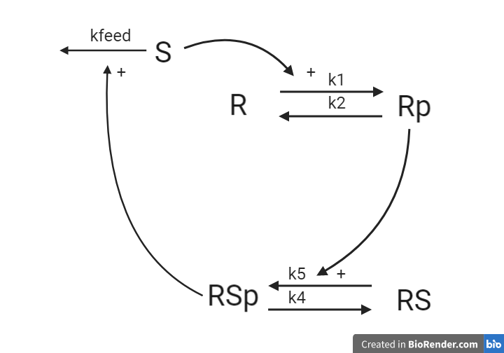
Hypothesis 2
This hypothesis is similar to the first one, but with some modifications. Here, the feedback-induced dephosphorylation of Rp (reaction 3 in the first model) is removed. Instead we add a feedback-dependent breakdown of the substrate S. This reaction is dependent on the states Rsp and S with a parameter kfeed(same name, but a different mode of action). These differences yield the following interaction-graph:
Implement hypothesis 2
Now, let us do the same thing again but for hypothesis 2.
Create a copy of your previous model file and implemented the changes in the hypothesis 2. Use the following values:
| Initial values | Parameter values |
|---|---|
| R(0) = 1 | k1 = 5 |
| Rp(0) = 0 | k2 = 20 |
| RS(0) = 1 | kfeed = 10 |
| RSp(0) = 0 | k4 = 15 |
| S(0) = 0 | k5 = 30 |
You should now be able to simulate the new model2 by only changing modelName and params in your Main script.
[ ] Checkpoint 3: Is the agreement between models and data convincing? Can we test quantitatively if it is good enough?
Testing models
Background
After implementing the two hypotheses into two models, you have two questions about your models:
Q1. How good are the models?
To better evaluate your models you want to test them quantitatively.
Let us first establish a measure of how well the simulation can explain data, referred to from now on as the cost of the model. We use the following formulation of the cost:
Where is the cost, given a set of parameters . and is experimental data (mean and SEM) at time , and is model simulation at time .
, is commonly referred to as residuals, and represent the difference between the simulation and the data. These are summed in the equation above, or rather, the squared residuals are summed. Note that the residuals in the equation above is also weighted with the SEM.
Q2. Are the models good enough?
Well, you see that they don't look like the data, but when are they are good enough?
There exists many statistical tests that can be used to reject models. One of the most common, and the one we will focus on in this lab is the -test. A -test is used to test the size of the residuals, i.e. the distance between model simulations and the mean of the measured data (Figure 2).
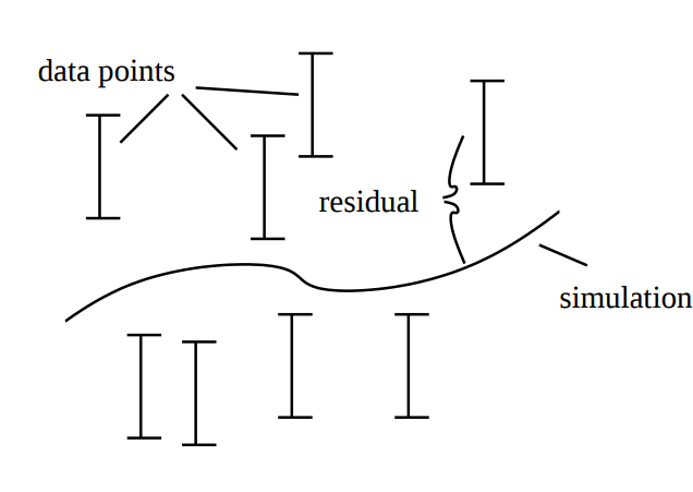
Figure 2: Residuals are the difference between model simulation and the mean of the measured data
For normally distributed noise, the cost function, , can be used as test variable in the -test. Therefore, we test whether is larger than a certain threshold. This threshold is determined by the inverse of the cumulative distribution function. In order to calculate the threshold, we need to decide significance level and degrees of freedom. A significance level of 5% (p=0.05) means a 5% risk of rejecting the hypothesis when it should not be rejected (i.e. a 5 % risk to reject the true model). The degrees of freedom is most often the number of terms being summed in the cost (i.e. the number of data points).
If the calculated cost is larger than the threshold, we must reject the hypothesis given the set of parameters used to simulate the model. However, there might be another parameter set that would give a lower cost for the same model structure. Therefore, to reject the hypothesis, we must search for the best possible parameter set before we use the -test. To find the parameter set with the lowest cost, we use optimization.
But first, we must find a way to calculate the cost. This is done using a cost function.
Calculate the cost
Create a function that takes the experimental data, parameter values and the model name as input arguments and returns the calculated cost as the output argument.
Note: You should use your already created SimulateExperiment function to do the simulation. Call your simulation function from inside the CostFunction to get the simulated values. The relationship between your functions are illustrated below.
Note: MATLAB interprets operations using *, /, ^ between vectors as vector operations. You likely want elementwise operations. This can be solved by introducing a dot . before any such operation (such as changing / to ./). Note that this is not an issue for +, -, if the vectors are of the same size.
Tip: You might have to transpose ySim when calculating the cost. This can be done by adding a ' after the variable (e.g. ySim')
You should now calculate the cost for both models using the default parameters. You should now only have to switch the value of modelName (or pass a long the name as an input argument to the cost function) in your script to get the cost for the other model.
Evaluate the cost
Now, you will try to reject the hypothesis with a -test.
Calculate the limit to when the model must be rejected. You can get a limit by using the function limit = chi2inv(0.95,dgf). Where 0.95 represents a p-value of 0.05 (1 - 0.05), and dgf is the degrees of freedom. Use the number of data points with non-zero SEM as the degrees of freedom: dgf = sum(SEM ~= 0, 'all').
Extra: Alternative interpretations of the limit and degrees of freedom
When selecting the degrees of freedom, there exists two major alternatives. The first is to set dgf = number of data points. The second is to set dgf = number of data points - number of identifiable parameters.
A third alternative could be to set limit = optimalCost + chi2inv(0.95,1) (note, dgf = 1).
If cost>limit, reject the model!
[ ] Checkpoint 4: Do you reject any of the hypotheses? Are there other statistical tests you can use?
Improving the agreement to data
Background
To do be able to test the hypothesis, we must find the best agreement between data and simulation. If the model is not good enough assuming we have the best possible parameters, the hypothesis must be rejected. It is possible to find this best combination of parameters by manually tuning the parameters. However, that would almost certainly take way too much time. Instead, we can find this best agreement using optimization methods.
An optimization problem generally consists of two parts, an objective function with which a current solution is evaluated and some constraints that define what is considered an acceptable solution. In our case, we can use our cost function as an objective function and set lower and upper bounds (lb/ub) on the parameter values as constraints. The problem formulation typically looks something like the equations below.
An optimization problem can be hard to solve, and the solution we find is therefore not guaranteed to be the best possible solution. We can for example find a solution which is minimal in a limited surrounding, a so-called local minimum, instead of the best possible solution – the global minimum (Figure 3). There are methods to try to reach the global minimum, for example you can run the optimization several times from different starting points and look for the lowest solution among all runs. Please note that there might be multiple solutions with equal values.
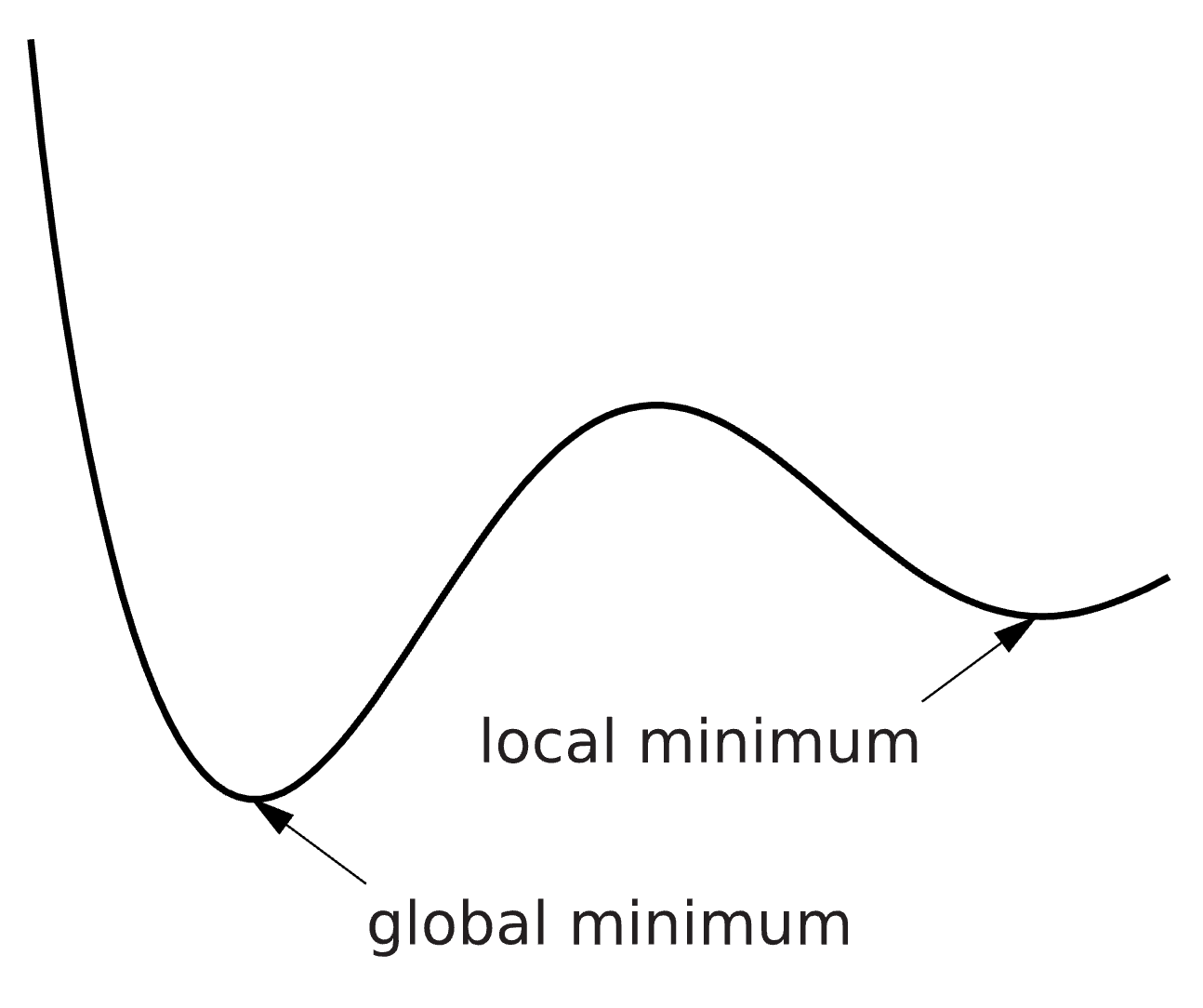
Figure 3: The difference between a local and a global minimum.
Furthermore, there exists many methods of solving an optimization problem. If a method is implemented as an algorithm, it is typically referred to as a solver.
Implement optimization
Now it is time to optimize the parameter values with respect to the agreement with the experimental data. In the end, your scripts should have a structure similar to the figure below.
Optimization solver* Refers to the optimization solver you will use (most likely eSS from the MEIGO toolbox).
f refers to the function used to evaluate a parameter set (typically CostFunction), x0 to the starting guess for the parameter values, lb and ub to the lower and upper bound for the parameter values.
Note also that not all optimization solvers require the same input, but in general they all require a function that can be used to evaluate a parameter set, a start guess of the parameter values (x0), as well as lower and upper bounds on what values the parameter can have.
Implementing the solvers from the MEIGO toolbox
Remember that you need to have the MEIGO toolbox installed
To use the solvers from the MEIGO toolbox, we must first define our problem.
x0 = params; %Define a set of starting parameter values

% Defining meigo problem
problem.f = 'CostFunction'; % The function used to evaluate the parameter values
problem.x_L = 1e-5*ones(1, length(x0)); % Sets the lower bound to 10^-5 for each parameter
problem.x_U = 1e5*ones(1, length(x0));% Sets the upper bound to 10^5 for each parameter
problem.x_0 = x0;  % Make sure that the orientation x_0 agrees with x_L and x_U
We must then set some options for the MEIGO optimization solvers. Below is an example, where you can play around with the values to see how they affect the optimization. Note that the best settings depends on each problem you are trying to solve. Thus, what you set now might not be the best settings for your future problems.
% Defining meigo options
opts.iterprint    = 1; % Set to 0 to disable printout of progress
opts.ndiverse     = 250; %'auto'; %100; %500; % auto = 10*nParams
opts.maxtime      = 1000; % In cess this option will be overwritten
opts.maxeval      = 1e5;

% Defining meio options for the local solver
opts.local.iterprint = 1; % Set to 0 to disable printout of progress
opts.local.solver = 'dhc'; %'dhc'; %'fmincon'; %'nl2sol'; %'mix'; %
opts.local.finish = opts.local.solver; % Use the same local solver as the global solver
opts.local.bestx = 0;
opts.local.tol = 3; % You probably want to move this down to 2 or 1 in your real projects
opts.local.use_gradient_for_finish = nargout(problem.f)>1; % You can ignore what this setting does for now, but it must be set.

% Define eSS specific options
opts.dim_refset   = 'auto'; %
The full details on the toolbox and all available options are available in the documentation.
Searching in log-space
It is often much faster to search for parameter values in log-space.
To do this, list all indices of the parameter vector that should be searched in log space. This is done by setting the opts.log_var to the list of indices to search in log-space: e.g., opts.log_var = [1:length(problem.x_L)] to search all parameter in log-space.
Using a good start guess
It is typically good idea to use a good start guess. If you are running multiple optimizations in sequence, consider using the previous best solution. One simple way to test if an optimization have already been run is to check if the results variable exists, and otherwise use a default value.
if exist('results','var') && ~isempty(results)
    x0 = results.xbest;
else
    x0 = params;
end
Running the optimization
Finally, we must select our algorithm and then run the optimization.
% Select algorithm and run the optimization
optim_algorithm = 'ess'; % 'ess'; 'multistart'; 'cess';
results = MEIGO(problem,opts,optim_algorithm, modelName, expData);
Note that the MEIGO function takes the problem definition, opts, and optim_algorithm as inputs, as well as all arguments to the function defined in problem.f (CostFunction in our case) in addition to the parameter values. In other words, the first argument sent to the cost function will always be the parameter set to test, and we do not have to specify explicitly that this argument should be sent to the cost function. Note that the order of the other arguments (modelName and expData) must be the same as in the cost function.
The results will be saved in the results variable. The best found parameter set is stored in results.xbest, and the best cost is stored in results.fbest.
Extra: Additional toolboxes and solvers
As mentioned, there exists multiple toolboxes. So far, we have noticed the best performance using the eSS solver from the MEIGO toolbox, but for reference you can read about some other toolboxes if you are interested.
Some alternatives (read about them with doc solver)
MATLAB's versions: particleswarm, simulannealbnd, fmincon,
IQM toolbox versions: simannealingIQM, simplexIQM
It is possible that not all solvers are equally good on all problems.
If you do not have a good start guess, particle swarm (which don't need a start guess) is probably a good start.
If you have a reasonably good start guess, it is probably a good idea to use a scatter search or a simulated annealing based solver.
Note, if you want to use the MATLAB solvers, you need to have the Global optimization toolbox.
Installing the global optimization toolbox
If you did not install the toolbox during MATLAB installation, search for "global optimization" in the add-ons explorer.
Enable passing one input variable to the cost function.
If you are using a solver not from the MEIGO toolbox, you will need to construct an anonymous function that can take only the parameter values as input, and pass along additional arguments to the cost function.
Most solvers can only call the cost function with one input variable (the parameter values). We must therefore update our script so that we only pass one input from the Main script to the cost function.
One way to bypass this limitation is to update the CostFunction to only accept one input and instead get the data and select model by either loading the data and model name in the cost function, or by getting them in as global variables. However, both of these methods have issues. A third (and better) alternative is to use an anonymous function. You can read more about anonymous functions here. Essentially, we create a new function which takes one input, and then calls CostFunction with that input as well as extra inputs.
How to implement an anonymous function:
Replace (in main_function):
cost = CostFunction(expData, modelName, params)
With:
func = @(p) CostFunction(expData, modelName, p)
cost = func(params)
Here, func acts as an intermediary function, passing along more arguments to the real cost function. Note that if expData is changed (after you have defined it), the output from func will not change. To do that, func must be redefined (as above).
An example with simulannealbnd
lb = [1e-5, 1e-5, 1e-5, 1e-5, 1e-5]
ub = [1e5, 1e5, 1e5, 1e5, 1e5]
[bestParam, minCost]= simulannealbnd(func, x0, lb, ub)
Searching in log-space
It is often better to search for parameter values in log-space. To do this, simply take the logarithm of the start guess and lower/upper bounds. Then, go back to linear space before the simulation is done in SimulateExperiment.
In Main:
x0=log(x0)
lb=log(lb)
ub=log(ub)
in SimulateExperiment:
param=exp(param)
Note that the simulation always have to get the "normal" parameters, if you pass along logarithmized parameters, some will be negative and the ODEs will be hard to solve (resulting in a CV_ERR_FAILURE error)
Tip 1: using multiple solvers
You can string multiple solvers together. E.g since particle swarm does not require a start guess, it can be used to find one and then pass it on to simannealing.
[bestParamPS, minCostPS] = particleswarm(func, length(lb), lb, ub)
[bestParam, minCost] = simulannealbnd(func, bestParamPS, lb, ub)
Tip 2: showing the progress while solving
If you want to see how the optimization progresses, you need to send in an options variable to the optimization algorithm. Below is an example for particleswarm. All MATLAB solvers (the IQM toolbox ones are a bit different) handles options in the same way, but note that the solver name has to be passed when setting the options.
options=optimoptions(@particleswarm, 'display','iter')
particleswarm(func, length(lb), lb, ub, options);
Saving the results
Nothing is worse than having found a good parameter set, only to overwrite it with a bad one, and then being unable to find the good one again. To avoid this, you should always save your results in a way that does not overwrite any previous results. Use MATLAB's save function.
save('filename.mat', 'variable')
Note: Change filename to the file name you want (e.g., 'model1 (123.456)'), and variable to the name of the variable you want to save (e.g. 'results'). The .mat specifies the format the variable should be saved as. The 'MAT' format is generally good to save workspace variables (such as the 'results').
The optimization solver return a structure results containing the results from the optimization. One of the results is ´results.fbest´ which is the best cost found during the optimization.
bestCost = results.fbest
Tip: Using the current time as file name
A good file name to use, that would not overwrite previous results would be to use the current time and date in the name. For this, you can use the MATLAB function datestr. The default layout of the time and date contains characters you can't use when saving a file. To avoid this, we pass along a second argument, with the desired format of the date string.
datestr(now, 'yymmdd-HHMMSS')
Or even better, with also the model name and the bestCost:
[modelName, ' opt(', num2str(bestCost), ')_' datestr(now, 'yymmdd-HHMMSS') '.mat']
Improve the optimization
Experiment with the solvers. What is the best fit you can get? How does it look if you plot the best parameter sets?
You should get costs for both models that are at least below 20 (likely even better, but let's not spoil that). Plot your best results, to make sure that nothing strange is happening with the simulations.
[ ] Checkpoint 5: Do you have to reject any of the models?
Model uncertainty
Background
If the cost function has a lower value than the threshold, we will move on and further study the behavior of the model. Unless the best solution is strictly at the boundary, there exists worse solutions than the best one, which would still be able to pass the statistical test. We will now try to find acceptable solutions, which are as different as possible. In this analysis, we study all found parameter sets that give an agreement between model simulation and experimental data – not only best parameter set. The parameter sets are used to simulate the uncertainty of the hypothesis given available data. This uncertainty can tell us things like: Do we have enough experimental data in relation to the complexity of the hypothesis? Are there well determined predictions (i.e. core predictions) to be found when we use the model to simulate new potential experiments?
Save all acceptable parameters (below limit)
The easiest way of doing this is to create a text file (filename.csv in this case), and write to that file every time the cost of a tested parameter set is below the limit (e.g. the chi2-limit). This you can do using fopen, which opens he file and creates a file identifier (fid) that can be passed to different functions.
In Main:
fid = fopen('filename.csv','a') % preferably pick a better name. a = append, change to w to replace file
----do the optimization ----
fclose(fid) % We need to close the file when we are done. If you forget this, use fclose('all')
In CostFunction:
Add the open file id fid as an input argument:
[cost] = CostFunction(expData, modelName, params, fid)
Write the parameter set to the file:
----simulate and calculate cost ----
if cost< limit
  fprintf(fid, [sprintf('%.52f, ',params) sprintf('%.52f\n',cost)]); % Crashes if no fid is supplied. See tip below. Note that the cost is saved as the last column
end
Remeber to also add the fid as an input to the optimization function back in your Main.
results = MEIGO(problem,opts,optim_algorithm, modelName, expData, fid);
Tip: Avoiding crashes if fid is not supplied
To not have the function crash if fid is not supplied, we can use “nargin”, which is the number of variables sent to the function. If we have said that fid will be the 4th input argument (see above), we can add another statement to the if-statement in the CostFunction.
if cost< limit && nargin==4
  fprintf(fid, [sprintf('%.52f, ',params) sprintf('%.52f\n',cost)]);
end
Run many optimizations
In order to gather many parameter sets to give us an estimation of the model uncertainty, re-run your optimization a few times to find multiple different parameter sets. Ideally we want to find as different solutions as possible. To do this the easy way, just restart your optimization a few times and let it run to finish. It might also be useful to start with different start guesses. Hopefully, running the optimization many times will find a reasonable spread of the parameter values. More optimizations will give an uncertainty closer to the truth. In the end, open your text file and check that there are a good amount of parameter sets in there.
Sample the saved parameters
Create a new “main” script
This new main script is for sampling your saved parameters and plotting. You can essentially copy your old Main script and use that as a base. We will not be optimizing anymore, so those lines can be removed.
Load your saved parameters
Import your .csv files using e.g load, readtable or dlmread
To convert from a table to array, use the function table2array.
Sample your parameter sets
For computational reasons, it is infeasible to plot all parameter sets. Therefore, we need to sample the parameter sets. There are multiple ways of sampling the parameter sets, where some are better than others. One way is to pick at random
It is likely reasonable to plot around 1,000 parameter sets in total.
Suggestion on function/variable names and structure:
[sampledParameters] = SampleParameters(allParameters)
A good way to select parameters
Use sortrows to sort based on the values in a column, then select some parameter sets with a fixed distance. Try picking ~100 sets. Then sort based on second column and repeat.
Some easy ways to select parameters
Pick indices at random
Use randi to generate ~1000 positions from 1 to the total number of parameter sets you have. E.g. ind=randi(size(allParameters,1),1,1000)
Pick indices with equal spacing
Use linspace to generate indices with equal spacing. Note, some values you get from linspace might not be integers. Therefore, round the values using round. E.g ind=round(linspace(1,size(allParameters,1),1000)).
Then, extract those parameter sets from allParameters.
sampledParameters=allParameters(ind,1:end-1); % last column is the cost
Plot model uncertainty
Use your simulation script to simulate your selected parameters. Plot model 1 with uncertainty in one color. Then, do the same thing for model 2, and plot in the same windows with another color. Lastly, plot the data. In the end, you should have both models and the data in one plot.
Suggestions on how to implement this:
Make a copy of PlotExperiment (perhaps named PlotExperimentUncertainty), and pass along sampled parameters and model names for both models. Then do either of the following:
1) Plot multiple lines, with different colors for the different models.
Note that this solution might be slower and/or more taxing on the computer resources.
Update the PlotExperiment function to take an extra input argument for color, and loop over your sampledParameters for one model with one color. The then repeat again for the next model with a different color.
Alternatively, create a new plot function and use your simulation script to simulate your selected parameters. Plot all the simulations as multiple lines in the same figure with the same color (one model = one color).
Then, do the same thing for model 2 and plot in the same windows.
Lastly, plot the data.
2) Find the maximal/minimal values and plot an area using `fill`
First, simulate all parameter sets and save the maximum and minimum value (ymin and ymax in the example below), then plot using fill. A simple way to do this is to first simulate any parameter set and set ymin and ymax to that value. Then, simulate all other parameter sets and update ymin and ymax if the simulation is either larger or smaller than the previous extreme. This can be done efficiently using logical indexing.
An example of how to implement the finding of the minimal and maximal values is shown below.
Note that it is probably a good idea to use a time vector of high resolution when simulating here if it is not already of a high resolution.
% Assumes the parameter sets are available in a variable named parameters, with rows for each parameter set
p0 = parameters(1,:);
[ysim0, timeSim] = SimulateExperiment(modelName, p0, time);
ymin = ysim0;
ymax = ysim0;

for i = 1:size(parameters,1)
    params = parameters(i,:);
    ysim = SimulateExperiment(modelName, params, time);
    smallerIdx = ysim < ymin;
    ymin(smallerIdx) = ysim(smallerIdx);
    largerIdx = ysim > ymax;
    ymin(largerIdx) = ysim(largerIdx);
end
Next, plot the simulation uncertainty by using the fill function in MATLAB. Note that fill creates a shape using the pairs in x and y, and always connects the first and last points. Therefore, to get a correct shape we must plot either the maximum or minimum value in reverse. This can be done using the function flip.
fill([time flip(time)], [ymin' flip(ymax')], 'k')
[ ] Checkpoint 6: Are the uncertainties reliable?
Predictions
Background
In order to see if the model behaves reasonable, we want to see if we can predict something that the model has not been trained on, and then test the prediction with a new experiment. Note that in order for the prediction to be testable, it must be limited in at least one point, often referred to as a core prediction.
Core predictions
Core predictions are well determined predictions that can be used to differentiate between two models. Such a differentiation is possible when model simulations behave differently and have low uncertainty for both models. Core predictions are used to find experiments that would differentiate between the suggested hypotheses and therefore, if measured, would reject at least one of the suggested hypotheses. The outcome could also be that all hypotheses are rejected, if none of the simulations agree with the new experiment. A core prediction could for example be found at one of the model states where we do not have experimental data, or at the model state we can measure, under new experimental conditions (extended time, a change in input strength etc.).
Experimental validation
The last step of the hypothesis testing is to hand over your analysis to the experimental group. The core predictions that discriminate between Model 1 and Model 2 should be discussed to see if the corresponding experiment is possible to perform. Now it is important to go back to think about the underlying biology again. What is the biological meaning of your core predictions? Do you think the experiment you suggest can be performed?
The outcome of the new experiment can be that you reject either Model 1 or Model 2, or that you reject both Model 1 and Model 2. What biological conclusions can we draw in each of these scenarios? What is the next step for you, the systems biologist, in each of these scenarios?
Design new experiment
Try to find a new experiment where the models behave differently.
Note, you must do the same thing in both models, so that you can differentiate them.
There are many things you can test in order to find a prediction where the models are behaving differently. Some alternatives are listed below.
Observing a different state
Even though the state we have been observing so far have been behaving in the same way in the two models, that might not be true for other states. Try to plot some different states and see if you can find one that behaves differently.
Manipulating the input signal
If we perturb the system a bit, it might be possible that the models will behave differently. One way could be to change the strength of the input signal (essentially changing the concentration of the substrate), or to manipulate it more complexly by for example changing the input at certain time points.
One easy way is to introduce another input argument to your SimulateExperiment function, which determines if a prediction should be simulated in addition to the original simulation (such as doPrediction). Then, if this prediction should be simulated, we simulate some additional time with some input.
if nargin > 3 && doPrediction
    ic = sim.statevalues(end,:); % Note that we now use the lastest simulation, not the steady state simulation
    ic(sIdx)=1;
    timePred = sim.time(end):0.01:4; % Simulate two additional time units (from 2 to 4)
    simPred = model(timePred, ic, params); % Replace [] with IC to use custom values
    ySimPred = simPred.variablevalues;

    ySim = [ySim; ySimPred(2:end)]; % Combine the two ysims to one vector. remove the double entry of ySim value at timepoint=2.0 which is present in ysim(end) and ySimPred(1)
    timeSim = [sim.time, simPred.time(2:end)]; % combine the two time vectors. Note that we append two row vectors, not two column vectors. We also remove the double entry of timepoint=2.0 which is present in sim.time(end) and simPred.time(1)
end
You probably also want to add a similar flag (doPrediction) to your PlotExperimentUncertainty function.
[ ] Checkpoint 7: What is a core prediction and why is it important? Do you think your prediction can be tested experimentally?
Evaluate your prediction
Background
You show the experimental group your predictions, and they tell you that they can do a second stimulation at time point 4, to set the amount of substrate to 1. They go about and perform the new experiment. Download the new experimental data from here or on LISAM.
Validation
Simulate the same prediction!
Note that you probably have to update your prediction to be this prediction (setting S = 1 at time = 4). If you followed the example with input manipulation above, you have to introduce an additional simulation between ranging from 2 to 4 before the prediction simulation, and update the prediction simulation with a new start time (4 to 6). In order words, the simulation should have the following overall order:
sim0 = simulate(0:1000)
get_ic
update_ic_S_to_1
sim = simulate(0:2)
get_ic
simPred0 = simulate(2:4)
get_ic
update_ic_S_to_1
simPred = simulate(4:6)

ysim = [sim; simPred0; simPred]
simTime = [sim.time, simPred0.time(2:end), simPred.time(2:end)]
Plot your prediction together with the validation data and evaluate the prediction with the cost and a -test as before.
Update the plot script to plot both the old simulation and experimental data, as well as the new prediction and prediction data.
For calculating the cost of the prediction, the best solution is likely to create a new cost function for the prediction, use the prediction by setting the doPrediction flag, and finding the overlapping time points. We can again use logical indexing to find the correct positions.
[ySim, timeSim] = SimulateExperiment(params, modelName, expData.time, doPrediction)% Do the prediction simulation using the updated SimulateExperiments function

predTimeIdx =  ismember(timeSim, expDataPred.time);

ySimPred = ySim(predTimeIdx);

% Calculate cost as before, now using the prediction simulation and predicition data.
[ ] Checkpoint 8: What do you want to tell the experimentalists?
Summary and final discussion
You have now gone through the computer lab, and it is time to look back upon what you have actually done, as well as to discuss some points that might be easy to misunderstand. Below are some questions to discuss with the supervisor.
Some summarizing questions to discuss
You should know the answers to these questions, but if you do not remember the answer, see this part as a good repetition for the coming dugga.
- Look back at the lab and, can you give a quick recap of what you did?
- Why did we square the residuals? And why did we normalize with the SEM?
- Why is it important that we find the "best" parameter sets when testing the hypothesis? Do we always have to find the best?
- Can we expect to always find the best solution for our type of problems?
- What are the problems with underestimating the model uncertainty?
- If the uncertainty is very big, how could you go about to reduce it?
- Why do we want to find core predictions when comparing one or more models?
This marks the end of the computer lab. We hope that you have learnt things that will be relevant in your future work!
Extras
The following sections regard things that might be relevant for you in the future but is outside of the scope of the lab. However, do feel free to come back here and revisit them in the future.
Introduction to profile-likelihood
In a profile-likelihood analysis, we plot one parameters value on the x-axis and the cost of the whole parameter set on the y-axis. Such a curve is typically referred to as a profile-likelihood curve. To get the full range of values for the parameter, it is common practice to fixate the parameter being investigated, by removing it from the list of parameters being optimized, and setting it explicitly in the cost function, and re-optimize the rest of the parameters. This is done several times, and each time the parameter is fixed to a new value, spanning a range to see how the cost is affected from changes in the value of this specific parameter (Figure 4). If the resulting curve is defined and passes a threshold for rejection in both the positive and negative direction (Figure 4A), we say that the parameter is identifiable (that is, we can define a limited interval of possible values), and if instead the cost stays low in the positive and/or the negative direction, we say that the parameter is unidentifiable (Figure 4B-D). This whole procedure is repeated for each model parameter.
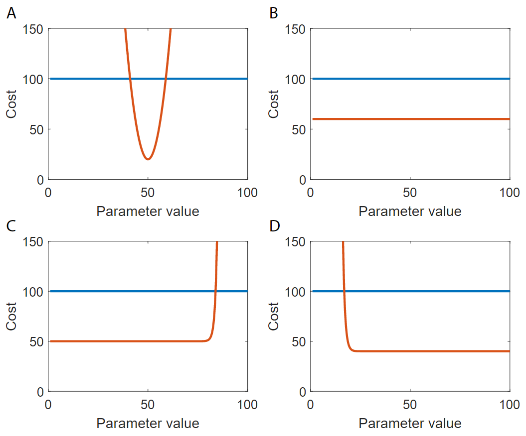
Figure 4: Examples of identifiable (A) and unidentifiable parameters (B-D). The blue line is the threshold for rejection, the red line is the value of the cost function for different values of the parameter.
In a prediction profile-likelihood analysis, predictions instead of parameter values are investigated over the whole range of possible values. Predictions cannot be fixated, like parameters can. Therefore, the prediction profile-likelihood analysis is often more computationally heavy to perform than the profile-likelihood analysis. Instead of fixation, a term is added to the cost to force the optimization to find a certain value of the prediction, while at the same time minimizing the residuals. Resulting in an objective function something like the following:
Again, the whole range of values of the predictions are iterated through. A prediction profile-likelihood analysis can be used in the search for core predictions.
A simple (but not ideal) approach
Here, we will not fixate one parameter at time and reoptimize, instead we will use the already collected data. This is worse than fixing the parameters, but we will do it for the sake of time. Furthermore, as opposed to the uncertainty plots before, we do not have to select some parameter sets, we can instead use all of our collected sets. The easiest way to do a profile-likelihood plot, is to simply plot the cost against the values of one parameter. Then repeat for all parameters.
To make it slightly more pretty, one can filter the parameters to only give the lowest cost for each parameter value. This can be done using the function unique. A good idea is likely to round your parameter values to something with less decimals. This can be done with round. Note that round only rounds to integers. To get a specific decimal precision, multiply and then divide the parameter values with a reasonable value. E.g.round(p*100)/100.
Changing figures
There are two main ways you can go about to change your figures to look nicer:
-
plot your figure first, and then make changes through the property inspector (Edit>Figure properties in the figure window), or
-
change the code for how you plot. This way, your figure will look like you want them to every time you run your plot scripts.
Some things that you can do to make your figure look nicer and easier to understand:
- Increase the linewidth (2 or 3 is usually good).
- Add a legend describing the different lines in your plot.
- Change the font and fontsize.
- Changing line style, so that lines can be distinguished without color.