TBMT42 Lab 2: Parameter estimation and model uncertainty analysis¶

Introduction¶

Welcome to the second computer exercise in the course TMBT42, Systems biology, Digital Twins and AI. In this computer exercise we will look at how we can combine mathematical models with experimental data to gain more insight into a biological system. This exercise will expand on the modelling workflow introduced in Lab 1. In Lab 1 you were introduced to how we formulate and analyse mathematical models from biological hypotheses. In this exercise we will examine how we can combine these models with experimental measurements to estimate values for the physiological parameters of the model. Furthermore, since biological systems are seldom described by absolute values, we will also look at how we can estimate plausible ranges of values for these parameters.These ranges of confidence intervals gives us an estimate of the model's uncertainty. Finally, we will look at how we can use the model to predict physiological variables that we have not measured.

How to pass (Click to expand)

Throughout this page you will find several questions. These questions are marked by green question boxes, like the one below:

Questions to relflect over

To pass this lab you should provide satisfying answers to these questions in your report.

Throughout this lab you will encounter code blocks that will help you preforme the different tasks of the lab. Understanding the code in each block and and analysing the output should help you answer the questions. The questions can be answered in a point-by-point format but each answer should be comprehensive, and adequate motivations and explications should be provided when necessary.

Please note that you are expected to include the figures generated by the code in your answers where it is applicable.

This version of the exercise is implemented as a Python version using the SciPy toolbox, running in an iPython notebook. This notebook can either be run online in Google Colab, or downloaded and run locally. If the download link does not work properly, right-click the link an "save link as ...", and save the ´.ipynb´-file in the location you want to run the lab.

Note: if you are running the lab in Google Colab, the first thing you should do is to save a copy of the notebook. To do this, press File > Save a copy in Drive (Arkiv > Spara en kopia på drive).

Also be aware that files created (e.g. for results later) are NOT saved when exiting the session, therefore always download backups of results. The notebook itself is saved between sessions.

About Python and notebooks¶

In a Python notebook, you can create either text or code cells. Text cells contain information like this, formatted using Markdown. Text cells can be edited by clicking twice in the box, and can be exited by clicking outside the text cell or by pressing save (differs based on notebook handler). Code cells contain actual code that can be run, typically by pressing a play button located on the top left of a code-cell when the mouse is kept over the cell (again it might differ a bit based on notebook handler). If running on Google Colab, note that the first time you run a cell (and after being idle for a longer time) you will be connected to server that runs the code, thus the first time you run a cell, you might have to wait a short while.

Finally, remember that Python uses so called "zero-based indexing", which means that the first position in for example lists have index 0, and the second position have index 1 and so on.

Importing necessary packages¶

Python is structured in such a way that only a core set of functions are available in the default setting. Additional useful functions are stored in optional packages. To access and use the functions in these packages, we need to explicitly import the packages. The first code section below imports the packages we need for this exercise. Please run the following code section by pressing the "play-button" located on the top left of a code-cell when the mouse is kept over the cell. After a few seconds a greed check-mark should appear to signal that the code block ran successfully.

import sys
import json
import csv
import random
import numpy as np
import math as m
import matplotlib.pyplot as plt
from scipy.integrate import odeint
from scipy.stats import chi2
from scipy.optimize import dual_annealing
from scipy.optimize import minimize

Now, you are ready to start the main tasks!

Background: The model and the experimental data¶

We will start by getting to know the system we will be working with. In this computer exercise we will work with the question of how blood pressure changes with age and which factors affect the blood preassure. This is a very important topic since Hypertension or high blood pressure is a major risk factor in several severe diseases. Below is a short summary of the system we will be working with.

Background (click me)

Hypertension is a condition defined as having a systolic blood pressure (SBP) above 140 mmHg and diastolic blood pressure (DBP) above 90 mmHg. Individuals suffering from hypertension run an elevated risk of developing further complications such as heart failure, aneurysms, renal failure, and cognitive decline. In addition, it is commonly observed that blood pressure increases with age, thus understanding what this relationship looks like is crucial for comprehending the associated risks and identifying factors that influence blood pressure.

When investigating blood pressure one has to keep in mind that the blood pressure depends on the cardiac cycle which is a dynamic process governed by the heart. This means that for each heart beat there will be an initial high pressure phase, when the heart contracts, followed by a low pressure phase when the heart is refilled. The systolic blood pressure (SBP), is a measure of the pressure exerted on arterial walls during the contraction phase of the heart. The diastolic blood pressure (DBP) reflects the pressure in the arteries when the heart is at rest between beats. Lastly, the mean arterial pressure (MAP) is a calculated value that provides an estimate of the average pressure exerted on the arterial walls throughout the cardiac cycle. The MAP takes into account both the SBP and DBP, incorporating the time spent in each phase of the cardiac cycle. MAP is subsequently an important parameter because it reflects the perfusion pressure necessary to deliver oxygen and nutrients to organs and tissues. It is particularly relevant in assessing overall cardiovascular health and evaluating the adequacy of blood flow to various organs.

Getting to know the experimental data¶

Experimental Data

For this exercise we will consider data for the SBP, the DBP and the MAP measured at different ages in a fictional population. Figure 1 below provides an illustration of this data, and the relationship between age and blood pressure. The blue data points represents the SBP, the orange data points corresponds to the DBP, and the green data points represents the MAP. The data shows th that on average the SBP increases somewhat linearly over the age span of 30 to 80 years, while the diastolic blood pressure increases at first but around age 50 it starts to decline. The MAP as expected represents the combined behaviour of both the SBP and DBP.

Figure 1: Figure 1 illustrates the experimental data for how the blood pressure increases with age for systolic blood pressure (SBP) in blue, diastolic blood pressure (DBP) in orange, and the mean arterial pressure (MAP) in green. The data is displayed as mean value with error bars indicating the standard error of the mean (SEM).

Defining the data¶

Typically, datasets are saved in spesific data files and which can then be loaded and analysed. In this case, we have inserted the values corresponding to the experimental data described above. The data has information regarding time points, mean values and standard deviations of the mean (SEM) for both SBP and DBP measurments.

The data is structured in what a so-called a dictionary (dict). In short, a dictionary structures data by connecting keys and values. The code below defines a dictionary data with the keys SBP and DPB. The corresponding values of SBP and DPB are themself dictionaries that contains the measurements for SBP and DBP respectively. Each of these dictionaries has the keys time, mean, and SEM with corresponding values being lists that contain the time points of the measurements, the mean values of the measurements, and the standard error of the mean (SEM) for each measurement respectively.

The last lines of the code below prints the content of the data-dictionary in a few different ways.

To make sure you understand how the data is structured, try to print different aspects of the data-dictionary yourself. For instansce what will the output of print(data['DBP']['mean']) be? You can edit and run the code block as many times as you want.

# Define the data---------------------------------------------------

data = {
    'SBP' : {
    'time': [30, 35, 40, 45, 50, 55, 60, 65, 70, 75, 80],
    'mean': [121.5424, 122.4240, 126.0144, 128.5636, 131.5991, 134.8431, 137.6694, 139.2801, 141.8642, 144.0324, 143.8378],
    'SEM': [2.6395, 2.6136, 3.4086, 3.6717, 4.4374, 4.6315, 4.7206, 4.6512, 4.8691, 5.6109, 5.0219]
    },
    'DBP' : {
    'time': [30, 35, 40, 45, 50, 55, 60, 65, 70, 75, 80],
    'mean': [77.9434, 79.1608, 81.4643, 82.3094, 82.4701, 82.2884, 81.3182, 79.4995, 77.6811, 76.1601, 73.9103],
    'SEM': [1.5577, 1.4522, 1.8223, 1.7906, 2.1005, 2.0920, 1.9503, 1.6569, 1.4524, 1.6829, 1.7161]
    }
}

print('All content of data:')
print(data)
print('\nKeys in data are:')
print(data.keys())
print('\nThe content of the "time" key of the SBP dictionary:')
print(data['SBP']["time"])

Plotting the data¶

Now that we have structured the data in a dictionary, we should visualize it. We do this by plotting the data using the package matplotlib and pyplot. In practice, we have shortened the name of matplotlib.pyplot package to plt when we imported the package earlier (import matplotlib.pyplot as plt). The code block below plots the data using the errorbar function. This function takes a few differnt arguments, first we define the x-values, y-values and errorbar sizes by the time, mean, and SEM feilds respectively- Secondly, we define that the points should not be connected by any line (linestyle='None'), the marker should be a circle (marker='o'), and that the legend value of each data series should correspond to the keys of the data-dictionary. We also set appropriate lables for the x- and y- axes with uinits.

To make the code reusable for later, we want to define a function that takes the data-dictionary as an input. This code block defines and then use this function to plot the data and show the figure.

def plot_data(data):
    for i in data.keys(): # loop over the keys of the dictionary
        plt.errorbar(data[i]['time'], data[i]['mean'], data[i]['SEM'], linestyle='None',marker='o', label=i) #for each key, plot the mean and SEM as errorbars at each time point
    plt.legend() # add a legend to the plot
    plt.xlabel('Time (min)') # add a label to the x-axis
    plt.ylabel('Blood pressure (mmHg)') # add a label to the y-axis

plot_data(data) # use the above-defined function to plot the data

Getting to know the model¶

Now that we have a better understanding for the data we will be working with lets take a closer look at how we can model blood pressure.

Model

The model used in this exercise is very simple and consists of two ordinary differential equations (ODEs) with a total of 6 parameters. The two states described by these ODEs are the SBP and DPB respectively.

\[\frac{d}{dt}(SBP)= \left(k_{1,SBP} + k_{2,SBP}*age\right)*\frac{SBP_0 - b_{SBP}}{117.86 - b_{SBP}}\]

\[\frac{d}{dt}(DBP)= \left(k_{1,DBP} - k_{2,DBP}*age\right)*\frac{DBP_0 - b_{DBP}}{75.85 - b_{DBP}}\]

The parameters \(k_{1,SBP}\) and \(k_{1,DBP}\) represents a combination of factors that are not significantly altered by the ageing process. These are typically inherent factors such as vascular tone or cardiac function.

The parameters \(k_{2,SBP}\) and \(k_{2,DBP}\) represents a combination of factors that are directly connected to the ageing. These could be factors such as increased arterial stiffness, reduced arterial compliance, and altered vascular function, all of which can contribute to the observed age-related change in blood pressure.

The parameters \(b_{SBP}\) and \(b_{DBP}\) represents the influence of factors that contribute to a person's baseline blood pressure level. These factors may include genetic predispositions, lifestyle choices, environmental influences, and chronic health conditions that impact blood pressure regulation.

\(SBP_0\) and \(DBP_0\) are the initial values for the two states respectively.

Lastly, the MAP is calculated as the difference between the SBP and the DBP, divided by 3 and added to the DBP.

\[ MAP = DBP + \frac{SBP - DBP}{3}\]

Define the model¶

Now let us take a look at how we define the equations described abve in Python, and how we can simulate the blood pressure model.

Firstly, we define the model as a function that takes the value of each state (state), the time points (t), and the parameter values (param) as inputs. This function then calculates and retuns the derivatives of SBP (ddt_SBP) and DBP (ddt_DBP). Nonte that in this case the inital values of the states (SBP0 and DBP0) are treated as parameter values

Run the code below to define the model.

# Define the model------------------------------------------------------------
def bp_model(state, t, param):

    # Define the states
    SBP = state[0]
    DBP = state[1]

    # Define the parameter values  
    k1_SBP = param[0]
    k2_SBP = param[1]
    k1_DBP = param[2]
    k2_DBP = param[3]
    bSBP   = param[4]
    bDBP   = param[5]
    SBP0   = param[6]
    DBP0   = param[7]

    # Define the model variables
    MAP = DBP + ((SBP-DBP)/3)
    age = t # time is the age of the patient

    # Define the ODEs
    ddt_SBP = (k1_SBP + k2_SBP*age)*((SBP0-bSBP)/(117.86-bSBP))
    ddt_DBP = (k1_DBP + k2_DBP*age)*((DBP0-bDBP)/(75.8451-bDBP))

    return[ddt_SBP, ddt_DBP]

Simulate and plot the model¶

To simulate the model that we have defined above we need to use a program that can numerically solve the ODEs we defined in our model function. For this exersice we will use the odeint function implemented in the scipy-module.

We also need to define some values for the model parameters and inital values for the states. The values that we will use for an inital simulation are specified in the table below. For the inital statevalues we'll assume resonable values of SBP and DBP for a healthy 30 year old.

Parameter values

Initial values	Parameter values
SBP(0) = 115	k1_SBP = 1
DBP(0) = 60	k2_SBP = 0
	k1_DBP = 1
	k2_DBP = 0
	bSBP = 100
	bDBP = 50

The code section below specifies these values as python lists. One list with two elements for the inital conditions (ic) of the states and one list with 8 elements for the parameter values (initial_parameterValues). Note that the last two entries in the parameter-values list are the two entries from the ic list.

We also need to define the time in years that we wish to simulate the model for. Here we define an array that goes from 30 to 81 in steps of 1, i.e. we will simulate the model from age 30 to age 81.

The final line prints the simulated values in two columns. The first column contains the simulated values for SBP and the second column contains the simulated values for DBP.

ic = [115, 60] #[SBP(0) = 115, DBP(0) = 60]
initial_parameterValues = [1, 0, 1, 0, 100, 50, ic[0], ic[1]] #[k1_SBP = 1, k2_SBP = 0, k1_DBP = 1, k2_DBP = 0, bSBP = 100, bDBP = 50]
t_year = np.arange(30, 81, 1)

sim = odeint(bp_model, ic, t_year, (initial_parameterValues,)) # Simulate the model for the initial parameters in the model file
print(sim)

Questions to reflect over

How does these simulated values compare with the data you plotted above?

Plotting the model simulation agreement with data¶

As you might have noticed it can be difficult to compare how well the model agree with the experimental data by just looking at the simulated values.

Therefore we want to create a function that can plot the model simulation. The function plot_Simulation is defined in the code section below. This function simulates the model, using odeint (like before) and plot each column of the sim variable as a line. The inputs to the plot function will therefore be the name of our model-function (bp_model), the parameter values (param), the inital condition (ic), and the time vector to simulate (t).

We can use the same varaibles for inital_parameterValues, ic, and t_year that we defined above.

Run the code section below to define and use the plot_simulation-function.

def plot_simulation(model, param, ic, t, state_to_plot=[0,1], line_color='b'):
    sim = odeint(model, ic, t, (param,)) # Simulate the model for the initial parameters in the model file
    stateNames = ['SBP simulation', 'DBP simulation'] # Define the names of the states
    colours = ['b', 'r'] # Define the colours of the lines
    for i in range(np.shape(sim)[1]): # loop over the number of columns in the sim array
        plt.plot(t, sim[:,state_to_plot[i]], label=stateNames[i], color = colours[i]) # The data corresponds to Rp which is the second state



plot_simulation(bp_model, initial_parameterValues, ic, t_year)
plot_data(data)

Questions to reflect over

How does the simulated values compare to the measured data?

Improving the agreement manually¶

The simulated values will depend on the parameter values, which means that if we change the parmater values and/or the inital conditions we will get a differend model simulation. If we assume that the model is an accurate representation of the biological system that generated the data, we only need to correctly estimate the parameter values to achive a good agreement between the model and the data.

The code section below allow you to change the inital conditions (ic) and the parameter values, and see how these changes affect the model simulation.

Try to find a combination of parameter values that improves the agreement to data.

Note that the k1-parametrs are idealy changed in incraments of 1 (i.e. -1, 0, 1) and the k2-parametrs are idealy changed in incraments of 0.01 (i.e. -0.01, 0, 0.01).

ic_test = [115, 60] #[SBP(0) = 115, DBP(0) = 60]
parameterValues_test = [1, 0, 1, 0, 100, 50, ic_test[0], ic_test[1]] #[k1_SBP = 1, k2_SBP = 0, k1_DBP = 1, k2_DBP = 0, bSBP = 100, bDBP = 50]


plot_simulation(bp_model, parameterValues_test, ic_test, t_year)
plot_data(data)

Questions to reflect over

Can you find a combination of parameters that aligns the model with the data?

Checkpoint and reflection¶

This marks the end of the first section of the exercise. Show your figure which shows how well the model agrees with the data.

Some Additional questions to reflect over

Why do we want the model simulation to agree with the data?
When is the agreement good enough?
Was it easy finding a better agreement? What if it was a more complex model, or if there were more data series?

Parameter Estimation - Evaluating and improving the agreement to data¶

Clearly, the agreement to data (for the initial parameter values) is not perfect, and as you might have notised manually adjusting the parameters can be quite challenging. In other words we would like a more structured way of using the experimental data to estimate the model's parameter values.

Background: What is parameter estimation?

Parameter estimation is the process of estimating what model parameter values create the behaviour described by the experimental data. To evaluate whether our model can describe the observed data we need to find the parameter values that creates a good agreement between the data and the model simulation. If the agreement between model and data is not good enough assuming we have the best possible parameters, the hypothesis must be rejected. While it is possible to find this best combination of parameters by manually tuning the parameters. This is an extremely labour intensive process and would almost certainly take way too much time. Especially for more complex models where non-linear dynamics are introduced between the model parameters and the model behaviour. Instead, we can find this best agreement using optimisation methods.

An optimisation problem generally consists of two parts, an objective function with which a current solution is evaluated and some constraints that define what is considered an acceptable solution. We will look at how we can formulate the objective function below. As for our constraints these depend a bit on what type of model we are using but for the most part it will suffice with a set of lower and upper bounds (lb/ub) on the parameter values as constraints. The optimisation problem can then typically be formulated as something a kin to the equations below.

\[ \begin{aligned} &min\ v=\ Objective\ function(\theta) \\ &subject\ to: lb<\theta<ub \end{aligned} \]

Where we are minimizing the value of the objective function \(v\) which will depend on the parameter values \(\theta\). With the constraints that \(\theta\) cannot be smaller than \(lb\), nor larger that \(ub\).

As the value of the objective function can scale non-linearly with the parameter values \(\theta\) the optimisation problem can be hard to solve, and the solution we find is therefore not guaranteed to be the best possible solution. We can for example find a solution which is minimal in a limited surrounding, a so-called local minimum, instead of the best possible solution – the global minimum. This relationship is visualised in Figure 2 where different sets of parameter values \(\theta\) yield different values of the objective function to form a landscape with various hills and valleys. There are methods to try to reach the global minimum, for example you can run the optimisation several times from different starting points and look for the lowest solution among all runs. Please note that there might be multiple solutions with equal values.

Furthermore, there exists many methods of solving an optimisation problem. If a method is implemented as an algorithm, it is typically referred to as a solver. Different solvers will use different techniques to find their way "downhill" in the landscape of the objective function, all attempting to reach the global minimum.

Figure 2: An illustration of how the objective-function value varies with different parameter values \(\theta\). The figure also highlights the difference between a local and a global minimum and how the different solutions correspond to a model simulation.

As stated above, we want to evaluate how well the agreement between our model simulation and the data really is. We can already do this qualitatively by inspecting the figure you've just made. However, in order to use the computational tools we have available we need a way to describe this agreement between model and data quantitatively, i.e. we would like to assign a number to how good the agreement is.

Defining a quantitative agreement to data

To better evaluate the model's agreement with data, we want to test it quantitatively. Let us first establish a measure of how well the simulation can explain data, also known as the cost of the model. We use the following formulation of this cost:

\[v\left(\theta\right)=\ \sum_{\forall t}\frac{{(y_t-\ {\hat{y}}_t\left(\theta\right))}^2}{{SEM}_t^2}\]

Where \(v(\theta)\) is the cost, given a set of parameters \(\theta\). \(y_t\) is the mean values of the data points and \(SEM_t\) is the standard error of the mean at each respective time point \(t\), and \({\hat{y}}_t\) is model simulation at time \(t\). Here, \(y_t-\hat{y}_t\left(\theta\right)\), is commonly referred to as residuals (Fig. 3), and represent the difference between the simulation and the data. In the equation above, the residuals weighted with the SEM values, squared and summed over all time points \(t\).

The residuals gives us the quantitative difference between the mean value of the data \(y_t\) and the simulated value \(\hat{y}_t\left(\theta\right)\) of each time point. Dividing the residuals by with the standard deviation \(\sigma\) , or SEM if mean values are used, ensures that data points that are well determined contributes more to the total cost of the fit. In other words, data points with small values of \(\sigma\)/SEM will yield a larger quotient and thus be weighted more when evaluating the quantitative model agreement ot the data. Lastly, squaring the weighted residuals ensures that all residuals has a positive contribution to the total cost. Since some residuals will be positive \(y_t \gt \hat{y}_t\left(\theta\right)\) and some will be negative \(y_t \lt \hat{y}_t\left(\theta\right)\) we don't want these different sings to cancel each other out. Thus by squaring the values all residuals will have a positive contribution to the total cost.

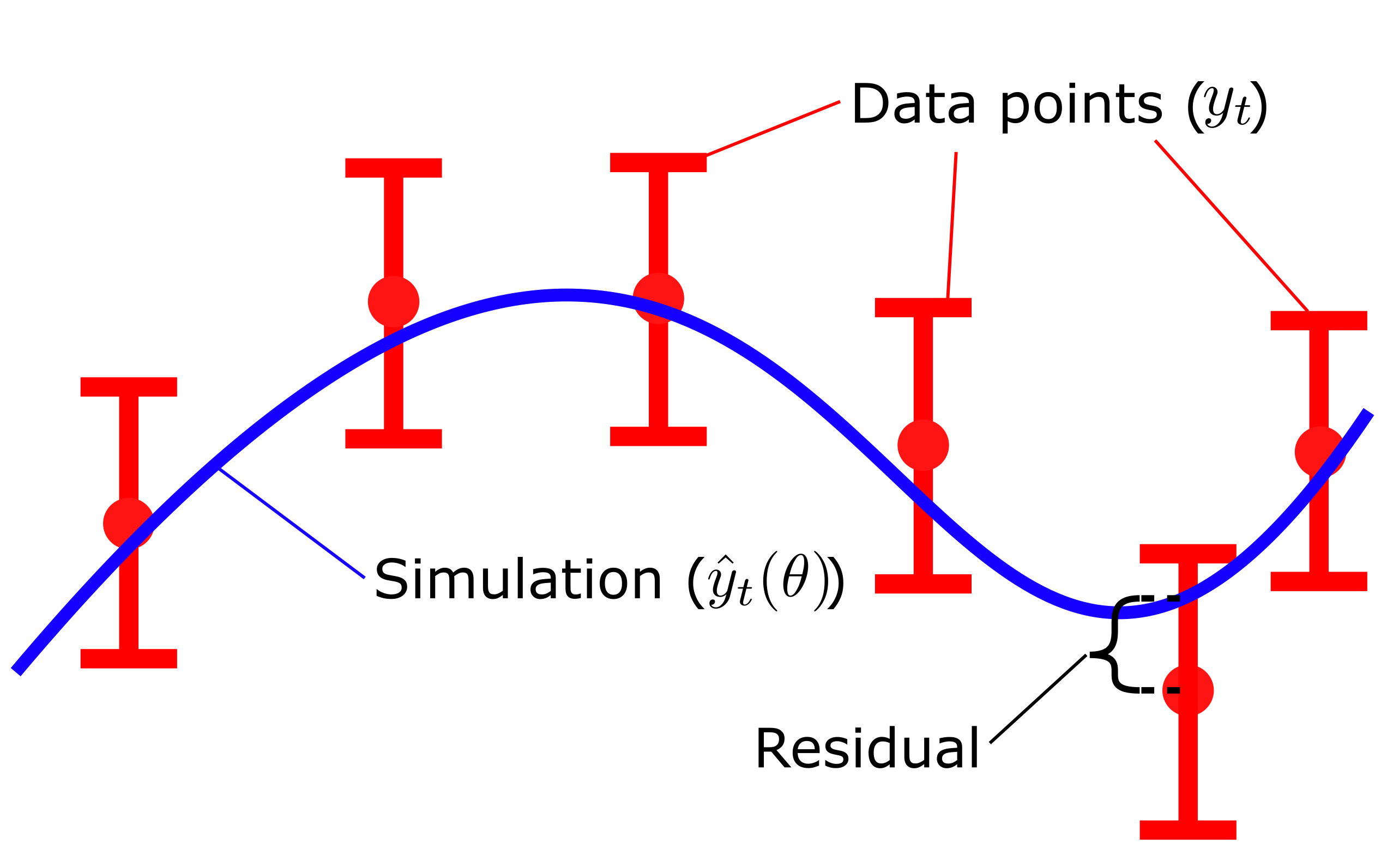
Figure 3: Residuals are the difference between model simulation and the mean of the measured data

The cost function, also know as an objective function, described in the section above is defined in the code block below.

This function takes the parameter values, model-function, and data-dictionary as input arguments. It runs a model simulation, simillarly to how we did before. We the apply the equation of the cost function to the SBP simulation/data and the DBP simulation/data respectively. Lastly, we add the respective costs together to get a total cost of the model's agreemnet with the data.

Note that when we run the simulation we use the time vector from the data-dictionary as the simulation time (t). In this way the simulated values (sim) will automatically be the same length as the data vectors. This means that we simply can subtract each element of the simulated values from the mean-data values (y_SBP - ysim_SBP).

Run the code block below to define the objective function.

# Define an objective function 
def objectiveFunction(parameterValues, model, data):
    t =  data['SBP']["time"]
    ic = parameterValues[6:8]
    sim = odeint(model, ic, t, (parameterValues,)) # run a model simulation for the current parameter values

    #--------------------------------------------------------------#
    ysim_SBP = sim[:,0]

    y_SBP = np.array(data['SBP']["mean"])
    sem_SBP = np.array(data['DBP']["SEM"])

    cost_SBP = np.sum(np.square((y_SBP - ysim_SBP) / sem_SBP))

    #--------------------------------------------------------------#
    ysim_DBP = sim[:,1]

    y_DBP = np.array(data['DBP']["mean"])
    sem_DBP = np.array(data['DBP']["SEM"])

    #---------------------------------------------------------------# 
    cost_DBP = np.sum(np.square((y_DBP - ysim_DBP) / sem_DBP))

    cost = cost_SBP + cost_DBP
    return cost

Calculating the cost of the initial parameter set¶

Now, let's calculate the cost for the model, given the initial parameter values, using the cost function we defined above (objectivefunction). Finally, let's print the cost to the output by using print and an f-string.

# use the obj function ------------------------------------------------------------
cost = objectiveFunction(initial_parameterValues, bp_model, data)
print(f"Cost of the model is: {cost}")

(spoilers) Self-check: What should the cost for the initial parameter set be if the model is implemented correctly?

If everything is implemented correctly, the cost for the initial parameter set should be approximately 731.55

Statistical test¶

With the cost function we can now quantitatively asses the agreement between the model simulation and the data. But how do we know if the solution is good enough? In other words what is a good cost?

There are several different statistical tests that can be used to reject models based on how well the model can describe given data. One of the most common, and the one we will focus on in this lab is the \(\chi^2\)-test.

The chi2-test

A \(\chi^2\)-test is used to test the size of the residuals, i.e. the distance between model simulations and the mean of the measured data

For data with normally distributed noise and a known standard deviation \(\sigma\), the cost function, \(v(\theta)\), will follow a \(\chi^2\) distribution, \(v(\theta)\) can thus be used as test variable in the \(\chi^2\)-test. Here, we test whether \(v(\theta)\) is larger than a certain threshold. This threshold is determined by the inverse of the cumulative \(\chi^2\) distribution function. In order to calculate the threshold, we need to decide significance level and degrees of freedom. A significance level of 5% (p=0.05) means a 5% risk of rejecting the model hypothesis when it should not be rejected (i.e. a 5 % risk to reject the true model). The exact number of degrees of freedom for this distribution can difficult to determine but for now we can use the number of terms being summed in the cost (i.e. the number of data points).

If the calculated \(\chi^2\)-test variable (i.e. the cost) is larger than the threshold, we must reject the null hypothesis for the given set of parameters used to simulate the model. The null hypothesis for the \(\chi^2\)-test is that the residuals (Figure 3) are small i.e. the model is in good agreement with the data. Rejecting this null hypothesis we say that the residuals are not small enough for us to believe that this specific model realisation and the data realisation of the system originates from the same distribution. This means that we do not believe that the system we are describing with our current model could have generated the measured data i.e. we are describing the wrong system.

The code section below performs a \(\chi^2\)-test and prints the conclusion based on the cost of the inital parameter values calculated above.

# Chi 2 test ---------------------------------------------------------------------

dgf = len(data['SBP']["mean"])*2
chi2_limit = chi2.ppf(0.95, dgf) # Here, 0.95 corresponds to 0.05 significance level

print(f"Cost of the model is: {cost}")
print(f"The Chi2 limit is: {chi2_limit}")
if cost < chi2_limit:
    print("The model is not rejected!")
else:    
    print("The model is rejected!")

Improving the agreement (manually)¶

As suspected, the agreement to the data was too bad, and the model thus had to be rejected. However, that is only true for the current values of the parameters. Perhaps this structure of the model can still explain the data good enough with other parameter values? To determine if the model structure (hypothesis) should be rejected, we must determine if the parameter set with the best agreement to data still results in a too bad agreement. If the best parameter set is too bad, no other parameter set can be good enough, and thus we must reject the model/hypothesis.

Try to change some parameter values to see if you can get a better agreement. It is typically a good idea to change one parameter at a time to see the effect of changing one parameter. If you did this in the previous section, you can reuse those parameter values.

ic_test = [115, 60] #[SBP(0) = 115, DBP(0) = 60]
parameterValues_test = [1, 0, 1, 0, 100, 50, ic_test[0], ic_test[1]] #[k1_SBP = 1, k2_SBP = 0, k1_DBP = 1, k2_DBP = 0, bSBP = 100, bDBP = 50]


plot_simulation(bp_model, parameterValues_test, ic_test, t_year)
plot_data(data)

cost = objectiveFunction(parameterValues_test, bp_model, data)

print(f"Cost of the model is: {cost}")
print(f"The Chi2 limit is: {chi2_limit}")
if cost < chi2_limit:
    print("The model is not rejected!")
else:    
    print("The model is rejected!")

Question to reflect over

Can you find a set of parameter values that is not rejected by the \(\chi^2\)-test?

Improving the agreement (using optimization methods)¶

As you have probably noticed, estimating the values of the parameters can be a hard and time-consuming work. To our help, we can use optimization methods. There exists many toolboxes and algorithms that can be used for parameter estimation. In this exersice we will use both a local and a global optimisation algorithm.

We'll start by looking at a local optimisation algorithm.

Local optimization¶

For the local optimisation we will use an algorithm called minimize from the SciPy toolbox. As you might remeber from the lectures, there are many differnt methods to approach an optimization problem and the minimize function have implementations for some of these differnt methods. In this example we will use a Nelder-Mead algorithm. The function is called in the following way: res = minimize(func, x0, args, method, bounds)

Description of the minimize function arguments

func - an objective function (we can use the cost function objectivefunction that we defined earlier),
x0 - a start guess for the parameter values,
args - any additional arguments needed for the objective function, in addition to the parameter values to test (in our case we need model, and data: objectivefunction(param, model, data))
method - specify which optimization method the minimize function should use,
bounds - upper and lower bounds of the parameter values,

The minimize function will return a dictionary (res) with the keys x corresponding to the best found parameter values, and fun which corresponds to the cost for the values of x.

By default the optimization implementation below will start at the default parameter values. If you have found good parameter values during the manual search you are free to use these as a start guess. Remember that the optimization problem is not guaranteed to give the optimal solution, therefore you might need to restart the optimization a few times (perhaps with different starting guesses) to get a good solution.

Run the code below to perfrom a local optimisation using the minimise-function.

Additional notes about optimization

Problematic simulations¶

Note that you might sometimes get warnings about odeint issues. If this only rarely happens, it is a numerical issue and nothing to worry about, but if it is the only thing happens, and you get no progress, something is wrong.

Computational time for different scales of model sizes¶

Optimizing model parameters in larger and more complex models, with additional sets of data, will take a longer time that in this exercise. In a "real" project, it likely takes hours if not days to find the best solution.

param_startGuess = [1, 0, 1, 0, 100, 50, ic[0], ic[1]] # You can can change the initial guess values
#parameter_OptBounds = np.array([(-1.0e6, 1.0e6)]*(len(param_startGuess)))
parameter_OptBounds = np.array([(-1.0e6, 1.0e6), (-1.0e6, 1.0e6), (-1.0e6, 1.0e6), (-1.0e6, 1.0e6),(50, 200),(20, 120),(70, 200),(50, 120)]) 

objFun_args = (bp_model, data)
niter = 0

res_local = minimize(objectiveFunction, param_startGuess, args=objFun_args, method='Nelder-Mead', bounds = parameter_OptBounds)
#print(res_local)
print(f"\nOptimized parameter values: {res_local['x']}\n")
print(f"Optimized cost: {res_local['fun']}")

print(f"chi2-limit: {chi2_limit}")


if res_local['fun'] < chi2_limit:
    print("The model is not rejected!")
else:    
    print("The model is rejected!")

Now, let's plot the solution you found using the optimization.

fig1 = plt.figure()
plot_simulation(bp_model, res_local['x'], res_local['x'][6:8], t_year)
plot_data(data)

Questions to reflect over

Do you think this model fit is good enought?
Do you think a better fit is possible? In that case, how could a better fit be achieved?
Does the choice of parameter start guess affect the outcome of the local optimisation?

Global optimisation¶

As you might have notised, local optimization algorithms leaves us with the risk of getting trapeped in local minima. To reduce the risk of this happening we could emplyo global optimization algorithms. Here we will use an algorithm called dual annealing from the SciPy toolbox. Which is an implementation of the simulated annealing method. It is called in the following way: res = dual_annealing(func, bounds, args, x0, callback)

Description of the dual annealing function arguments

func - an objective function (we can use the cost function fcost defined earlier),
bounds - bounds of the parameter values,
args - arguments needed for the objective function, in addition to the parameter values to test (in our case model, initial conditions and data: fcost(param, model, ic, data))
x0 - a start guess of the parameter values (e.g. param_guess_M1),
callback - a "callback" function. The callback function is called at each iteration of the optimization, and can for example be used to print the current solution.

Simillarly to the minimize function, the dual annealing function also returns a dictionary (res) with the keys x corresponding to the best found parameter values, and fun which corresponds to the cost for the values of x. However, unlike minimize, the dual annealing function also requires a callback function as an input argument. There fore we start by defining this callback funtion. This basic callback function simply prints the current objective function value (cost) to the output.

Run the code below to define the callback function.

# define a callback function that will be called at each iteration of the optimization algorithm    
def callback_fun(x,f,c):
    global niter
    if niter%1 == 0:
        print(f"Iter: {niter:4d}, obj:{f:3.6f}", file=sys.stdout)
    niter+=1

Run the code below to run the global optimization. Note again that the parameter values start guess is set to the default values. Feel free to change these as you se fit.

param_startGuess = [1, 0, 1, 0, 100, 50, ic[0], ic[1]]
#parameter_OptBounds = np.array([(-1.0e6, 1.0e6)]*(len(param_startGuess)))
parameter_OptBounds = np.array([(-1.0e6, 1.0e6), (-1.0e6, 1.0e6), (-1.0e6, 1.0e6), (-1.0e6, 1.0e6),(50, 200),(20, 120),(70, 200),(50, 120)]) 
objFun_args = (bp_model, data)
niter = 0

res_global = dual_annealing(func=objectiveFunction, bounds=parameter_OptBounds, args=objFun_args, x0=param_startGuess, callback=callback_fun) # This is the optimization
#print(res_global)
print(f"\nOptimized parameter values: {res_global['x']}\n")
print(f"Optimized cost: {res_global['fun']}")

print(f"chi2-limit: {chi2_limit}")

if res_global['fun'] < chi2_limit:
    print("The model is not rejected!")
else:    
    print("The model is rejected!")  


fig2 = plt.figure()
plot_simulation(bp_model, res_global['x'], res_global['x'][6:8], t_year)
plot_data(data)

Questions to reflect over

How does the model fit after the global optimization compare to the model fit following the local optimization?
Do you think that we have found the global optimum? Why/Why not?
Does the choice of parameter start guess affect the outcome of the global optimisation?

If running in Google Colab: remember to save the best solution you have found before exiting the session! The box below describes how to save the best solution from the global optimisation to a file that you can then download. You can find the file under the "Files"-tab on the left-hand side of the notebook. Right-click the optimized_parameters.json' file and select download.

Saving/loading parameters

After the optimization, the results is saved into a JSON file. Remember, if you run on Google Colab, the files will not be saved when you disconnect from the server. You can run the code below to save the best solution from the global optimisation to a file that you can then download.

file_name = 'optimized_parameters.json'  # You can change the file name if you want to.

with open(file_name,'w') as file:#We save the file as a .json file, and for that we have to convert the parameter values that is currently stored as a ndarray into a traditional python list
    json.dump(res_global['x'].tolist(), file)

If you later want to load the parameter set you can do that using the code snippet below. Remember to change optimized_parameters.json to the right file name. The loaded file will be a numpy array, but the code also stores this in a dictionary, where the parameter values can be accessed using results['x']

file_name = 'optimized_parameters.json' # Make sure that the file name is the same as the one you used to save the file

with open(file_name,'r') as file:
    optimal_ParameterValues = np.array(json.load(file))

res_global['x'] = optimal_ParameterValues # To ensure the following code will work as intenden, We replace the parameter values with the ones we just loaded from the file

Checkpoint and reflection¶

Questions to reflect over

Why do we want to find the best solution?
Are we guaranteed to find the global optimum?
Should the model be rejected?
What can we learn from the estimated parameter values?

Estimating model and parameter uncertainty¶

Now we have used the data for our system, here how the blood pressure changes with age, to create an estimation of what the parameter values of our model could be. This means that if we believe the data, we should also believe that our estimated value for e.g. \(k_{2,SBP}\) constitutes a reasonable value for the combination of factors that are directly connected to the ageing of our population. However, this solution is only one out of a multitude of possible solutions, all of which would pass the \(\chi^2\)-test. Since we can only make a meaningful conclusion regarding the model when we reject the model, we cannot claim that the solution we found are better than any other solution that also passes the \(\chi^2\)-test. Hence, what we really want is the distribution of all parameter values that result in an acceptable model behaviour (Figure 4). In this next section we will look at a few different approaches to estimates such distributions, and what can we learn about the system by analysing the distributions of acceptable model behaviours.

The importance of parameter uncertainty

As we have seen, in the field of systems biology, mathematical models play a crucial role in interpreting complex biological phenomena. Our models often contain various parameters representing biological characteristics such as different factors that affect the blood pressure. However, due to experimental limitations, inherent biological variability, and other sources of uncertainty, these parameters can rarely be known with absolute precision. This is why studying parameter uncertainties is crucial in systems biology.

Studying parameter uncertainties allows us to quantify the reliability of our model predictions. It is important to acknowledging that our models are not absolute but rather range within certain confidence intervals. Furthermore, understanding how sensitive the models are to variations in parameters can help identify key drivers of biological behaviour. This can inform experimental design, by focusing efforts on measuring the parameters that matter most, and lead to more robust and reliable predictions.

Moreover, a deep understanding of parameter uncertainties can reveal which parts of the system are well-defined and which parts are less known. This knowledge can be utilized to improve experimental designs, enhance the model by incorporating more data or refining assumptions, and ultimately increase our understanding of the biological system at hand. In this way, the study of parameter uncertainties not only bolsters the validity of systems biology models, but also acts as a guide for future research efforts.

Figure 4: An illustration of how the model uncertainty correlates to the objective-function landscape and the \(\chi^2\)-test. All parameter solutions that yields an objective function value that is below the \(\chi^2\)-threshold (blue shaded area) correspond to a collection of acceptable model simulation (blue shaded simulation)

Identifiable and unidentifiable parameters¶

The terms "identifiable" and "unidentifiable" are sometimes used to describe whether it's possible to uniquely determine these parameters based on the available data.

An "identifiable" parameter is one for which a unique estimate can be found from the data. That is, there is narrow range of parameter values that the can describe the data. The parameter can be well determined given the experimental data. This doesn't mean that we've necessarily found the true value of the parameter (due to experimental noise, model assumptions etc.), but rather that no other parameter values can produce a better fit to the data.

On the other hand, an "unidentifiable" parameter is one for which a wide range of different values could equally well fit the data. In other words, we can't pinpoint a unique estimate for the parameter from the data because several different parameter values produce essentially the same model behaviour. Unidentifiable parameters can present challenges in model calibration, as they lead to uncertainty in model predictions.

Markov Chain Monte Carlo (MCMC) sampling¶

Background: MCMC sampling

Markov Chain Monte Carlo (MCMC) methods are a class of algorithms in computational statistics used for sampling from a specific probability distribution. Monte Carlo sampling is a statistical technique that works by generating a large number of random samples from a probability distribution, and then approximating numerical results based on the properties of these samples. It's essentially a way to make numerical estimates using randomness. MCMC sampling expands on these concepts by selecting samples such that the next sample is dependent on the existing samples, creating a so called Markov chain. This will allows the algorithm to hone in on the quantity that is being approximated from the distribution, this is especially useful for problems with a large number of variables.

As a very simplified example, Imagine we have a large jar filled with marbles of different colours and we want to figure out what percentage of the marbles are red, blue, green, yellow, etc.. In other words, we want to find the distribution of coloured marbles in the jar. Imagine also that the jar is to large to count the marbles one by one. The principles of MCMC sampling could be used to estimate this colour distribution. We can construct a simple algorithm for solving this task:

You reach into the jar and select a marble at random. You record the colour and put the marble back in the jar.
You, again at random, pick another marble from the jar. If it's the same colour as the previous one, we put it back and pick another one. If it's a different colour, we record its colour and put it back in the jar. This "choosing based on the last choice" is the "Markov Chain" part.
We repeat step 2 a lot of times, thousands or millions of times. This is the "Monte Carlo" part, using repeated random sampling to obtain results.
Finally, we look at the colours we recorded. The proportion of each colour in our records gives us an estimate of the proportion of each colour in the jar.

The more samples we draw (the more marbles we pull out), the closer our estimated distribution gets to the actual distribution.

Please note that this is a very simplified analogy. Real MCMC methods can get quite complex, particularly when it comes to determining the rules for when to accept or reject the next sample, but the general idea remains the same.

For our purposes, we can use MCMC sampling to estimate the distribution of our model parameters or a specific model behaviour. Let's say that we want to approximate the parameter distributions that allow our model to explain the data. We can then use a MCMC sampling algorithm to select different parameter sets. We can then use a similar cost function as in the previous section to evaluate if the selected parameters describe the data adequately well, and if so we record the selected parameter set and move on. Thus by gathering enough samples, we can get an approximation of the possible parameter values that allow the model to still explain the data.

We will look at how to implement a simple MCMC sampling method. The following code implements a very simple Metropolis-Hastings algorithm for MCMC sampling. While you do not have to understand the exact details of the code below, please make some effort to see if you can identify the main principles of the MCMC sampling. If you have any questions please do not hesitate to ask the supervisor.

Run the code below to define the MCMC algorithm.

def target_distribution(x): # DEfine the target distribution you want to sample from, here we use the exponental of the objective function
    return np.exp(-objectiveFunction(x, bp_model, data))

def metropolis_hastings(target_dist, init_value, n_samples, sigma=1):
    samples = np.zeros((n_samples, len(init_value)))
    samples[0,:] = init_value
    burn_in = 100 # the burn-in represents the number of iterations to perform before adapting the proposal distribution
    dgf = len(data['SBP']["mean"])*2

    for i in range(1, n_samples):
        current_x = samples[i-1,:] # get the last sample
        if i < burn_in:# For the burn-in iterations, use a fixed candidate distribution, here a normal distribution.
            proposed_x = np.random.normal(current_x, 1) # calculate the next candidate sample (proposed_x) based on the previous sample.
        else: # After the burn-in period, use the covariance of past samples to determine the variance of the candidate distribution
            sigma = np.cov(samples[:i-1,:], rowvar=False)
            proposed_x = np.random.multivariate_normal(current_x, sigma) # calculate the next candidate as a random perturbation of the previous sample, with sigma based the covariance of all previous samples.

        acceptance_ratio = target_dist(proposed_x) / target_dist(current_x) # calculate the acceptance ratio, i.e the ratio of the target distribution at the proposed sample to the target distribution at the last sample

        # Accept or reject the candidate based on the acceptance probability. 
        # This probability is based on if the objective function value of the candidate vector in relation to the objective function value of the previous sample. 
        if np.random.rand() < acceptance_ratio:  # Accept proposal with probability min(1, acceptance_ratio)
             #if the proposed parameter values vector is accepted check if the correspondign model fit is acceptable. 
            if objectiveFunction(proposed_x, bp_model, data) < chi2.ppf(0.95, dgf): 
                current_x = proposed_x # if the model fit is acceptable, update the current parameter values to the proposed parameter values

        samples[i,:] = current_x # store the current parameter values in the samples array

    return samples

Now let's run the above-define algorithm. We will start the sampling from the optimal parameters obtined from the global optimisation res_global[x]. We will also need to set the number of samples we want to use. Typically we would want the number of samples to be high (> 1 000 000) but will more time. Therefore, in the intreset of time, we will start with 10 000 samples.

Run the code below to run the MCMC-algorithm and plot the sampled parameter distribution as histograms.

init_value = res_global['x']
n_samples = 10000

# Running the Metropolis-Hastings algorithm
samples = metropolis_hastings(target_distribution, init_value, n_samples)

## Plot the results
parameter_names = ['k1_SBP', 'k2_SBP', 'k1_DBP', 'k2_DBP', 'bSBP', 'bDBP', 'SBP0', 'DBP0']  # Define the names of the parameters

fig4, ax, = plt.subplots(2,4)
for i in range(len(init_value)):
    ax[m.floor(i/4),i%4].hist(samples[:,i], bins=30, density=True, alpha=0.6, color='g')
    ax[m.floor(i/4),i%4].title.set_text(parameter_names[i])
    ax[m.floor(i / 4), i % 4].set_xlabel('Parameter value')  # Set x-label for each subplot

plt.suptitle('Metropolis-Hastings algorithm')

fig4.set_figwidth(20) # set the width of the figure
fig4.set_figheight(12) # set the height of the figure

Question

What can you learn from observing the parameter distributions?

Please note that the implementation of the MCMC sampling algorithm that is presented above is still fairly rudimentary and does not sample the parameter space in a comprehensive fashion. Rather it is a simpler implementation for teaching the core principles of MCMC sampling for the purposes of this computer exercise. A ture MCMC sampling would require a more complex sampling algorithm and a higher number of samples. Such an analysis would also take more time than we have for this computer exercie. However, the parameter distributions for such a comprehensive MCMC-sampling have been prepared beforehand and the results are avilable for you to analyse. The following piece of code loads the prepared sample file and plots the fully sampled parameter distributions. You can download the pre-loaded MCMC-results file here. Download the zip file and unpack it to your working directory.

If you are running on Google colab you'll need to download, and unzip the the file. Then upload the TBMT42_Lab2_MCMC_results.json to the drive.

with open('TBMT42_Lab2_MCMC_results.json','r') as file:
    MCMC_results = np.array(json.load(file))

fig4, ax, = plt.subplots(2,4)
for i in range(len(init_value)):
    ax[m.floor(i/4),i%4].hist(MCMC_results[:,i], bins=30, density=True, alpha=0.6, color='g')
    ax[m.floor(i/4),i%4].title.set_text(parameter_names[i])
    ax[m.floor(i / 4), i % 4].set_xlabel('Parameter value')  # Set x-label for each subplot

plt.suptitle('Full MCMC results')
fig4.set_figwidth(20)
fig4.set_figheight(12)

Question

How does the fully sampled distributions compare to thoes produced by the simple Metropolis-Hastings algorithm?

Profile Likelihood¶

Profile Likelihood (PL) analysis is a computational approach used in model-based analysis to estimation of confidence intervals for parameters in a model. Profile likelihood is often used in the field of systems biology and other areas that employ complex mathematical models. Here we will look at two versions of a profile likelihood analysis. To start with, we will look at what is know as a partial- ,or some times, reverse Profile Likelihood. The full profile Likelihood analysis is introduced in more detail in the section below.

Reversed Profile Likelihood¶

Background: Reverse Profile Likelihood

The reversed, or partial, profile Likelihood is as the name suggests not as comprehensive but less computationally demanding, compared to a full profile likelihood analysis.

The main idea of a PL-analysis is that we can utilize an optimization algorithm to actively explore the highest and lowest permissible values for a particular model parameter without exceeding the established \(\chi^2\)-threshold. Essentially, each parameter should have some wiggle room to vary from the optimal solution before it pushes the result beyond this threshold. This range of variation for a parameter, while still contributing to an acceptable model solution, is sometimes referred to as the parameter's profile in relation to the likelihood (or cost) function.

Some parameters may have a broad range because changes can be offset by other parameters. On the other hand, for some parameters, the acceptable values range will be narrow, implying that these parameters significantly influence the model's behaviors.

Since the optimization solvers we utilized in the previous section aim to identify the parameters that minimize the given objective function, these algorithms can be repurposed to find the smallest (and largest) value for a specific parameter. If we perform this optimization for each parameter, we can establish confidence intervals for all acceptable parameter values in our model.

Figure 5: an illustration of a parameters Likelihood profile and how it relates to the maximal and minimal acceptable values for the parameter

Redefine the objective function¶

If we want to use an optimisation algorithm to find the minimum or maximum value for a certain parameter we want an objective function that reflects this purpose. To design such an objective function we need 3 addition inputs argument, compared to our previous objective function. We neen information regarding which parameter we are maximising/minimising, we need to know if we are maximising or minimising, and we need to know the \(\chi^2\)-threshold we should stay under. The following function is an example of what such an objective function might look like.

This function calculates the cost using the original objective function. The function then returns the parameter values of the parameter indicated by the parameterIdx variable. parameterIdx is a scalar value with the index of the parameter we want to maximise or minimise. The input variable polarity is either \(1\) or \(-1\) and indicates if we are maximising or minimising the parameter value. Most optimisation algorithm aim to minimize their objective function however, by multiplying the output value by \(-1\) we are effectively maximising the objective function value. Hence, if polarity = 1 we are minimising the parameter value, but if polarity = -1 we are maximising the parameter value.

Lastly, the function contains an if clause that kicks in if the cost is larger that the threshold i.e. we have an unacceptable solution. If this is the case we add a penalty term to the output value v. This penalty term will be exponentially proportional to how much above the threshold the current solution is.

def objectiveFunction_reversePL(parameterValues, model, Data, parameterIdx, polarity, threshold):
    # Calculate cost with original objective function
    cost = objectiveFunction(parameterValues, model, Data)

    # Return the parameter value at index parameterIdx.
    # Multiply by polarity = {-1, 1} to swap between finding maximum and minimum parameter value.
    v = polarity * parameterValues[parameterIdx]

    # Check if cost with the current parameter values is over the chi-2 threshold
    if cost > threshold:
        # Add penalty if the solution is above the limit.
        # Penalty grows the more over the limit the solution is.
        v = abs(v) + (cost - threshold) ** 2

    return v

The algorithm for the reversed profile likelihood analysis follows these steps:

Loop over all parameters in the model.
For each parameter: loop over the ploarity
For each parameter and polarity: run an optimisations with the modified objective function (objectiveFunction_reversePL).
Save the result of the optimisation.

The algorithm will result in two optimisations for each parameter, one to maximise the parameter value, and one to minimise the parameter value. For this optimisation we'll want to use a global algorithm that can use our optimal parameter values as a start guess. Here we'll use the same dual_annealing optimisation algorithm that we used previously.

Run the code below to run the reversed PL algorithm.

# Set up
param_startGuess = res_global['x']

#parameter_OptBounds = np.array([(-1.0e6, 1.0e6)]*(len(param_startGuess)))
parameter_OptBounds = np.array([(-1.0e6, 1.0e6), (-1.0e6, 1.0e6), (-1.0e6, 1.0e6), (-1.0e6, 1.0e6),(50, 200),(20, 120),(70, 200),(50, 120)]) 
parameter_bounds = np.zeros((len(param_startGuess),2))

dgf = len(data['SBP']["mean"])*2
threshold = chi2.ppf(0.95, dgf) # Here, 0.95 corresponds to 0.05 significance level 

# Running the actual algorithm 
for parameterIdx in range(len(param_startGuess)):
    for polarity in [-1, 1]:
        objFun_args = (bp_model, data, parameterIdx, polarity, threshold)
        niter = 0
        res_revPL = dual_annealing(func=objectiveFunction_reversePL, bounds=parameter_OptBounds, args=objFun_args, x0=param_startGuess, callback=callback_fun) # This is the optimization
        parameter_bounds[parameterIdx,max(polarity,0)] = res_revPL['fun']

Since we have used the polarity = -1 to determine the maximal value of our parameters (by minimising the negative value of the objective function) the values in the first column of parameter_bounds will be negative. Therefore we want to take the absolute value of these values to get the estimation of the maximal value.

parameter_bounds[:,0] = abs(parameter_bounds[:,0])  # Make sure that the upper bounds are positive

print("Estimated parameter bounds:")
print(parameter_bounds)

We can now plot the estimated parameter bounds. There is no one right way to do this but since we want to compare to the results of the PL analysis to the results of the MCMC-sampling, let us plot the parameter bounds for each parameter. The code below, plots the estimated PL-bounds as vertical red lines ontop of the MCMC histograms from earlier.

Run the code below to generate these plots.

# Plot the results of the reverse profile likelihood analysis ----------------------------------------------------------

fig4, ax, = plt.subplots(2,4)
for i in range(len(parameter_bounds)):
    ax[m.floor(i/4),i%4].hist(MCMC_results[:,i], bins=30, density=True, alpha=0.6, color='g')
    ax[m.floor(i/4),i%4].plot([parameter_bounds[i,:],parameter_bounds[i,:]],[[0, 0],[ax[m.floor(i/4),i%4].get_ylim()[1], ax[m.floor(i/4),i%4].get_ylim()[1]]], color='r')
    ax[m.floor(i/4),i%4].title.set_text(parameter_names[i])
    ax[m.floor(i / 4), i % 4].set_xlabel('Parameter value')  # Set x-label for each subplot

fig4.set_figwidth(20)
fig4.set_figheight(12)
plt.show()

Questions to reflect over

How does the estimated parameter bounds compare to the MCMC-sampling distrbutions?
What could be an explination for any observed differnences?

While the partial or reversed profile likelihood analysis above can be used to estimate the confidence intervals of the parameter values within a reasonable computational time. We would still be interested in analysing the full likelihood profile thus we will now look at what this means and how we can implement a full Profile likelihood analysis.

Full Profile Likelihood analysis¶

Now that we have done the partial profile likelihood we'll look at doing a full profile likelihood analysis. The drop-down section below goes into more detail of what this analysis entails.

Background: Full Profile Likelihood

The concept behind a profile likelihood analysis involves exploring how well the model fits the data as each parameter is varied, while optimizing the other parameters. Essentially, for each value of the parameter of interest, the values of the other parameters that maximise the likelihood (minimises the cost) are found. This gives a "profile" of the likelihood function for the parameter of interest. In other words one parameter is fixated at a specific value, while all other parameters are re-optimised. Then we step the fixated parameter away from the optimal value, re-optimising all other parameters for each step.

By creating a range of acceptable values (usually based on a \(\chi^2\)-threshold), a confidence interval for each parameter can be determined. This process is then repeated for each parameter in the model.

The advantage of the profile likelihood method is that it takes into account the correlations between parameters and the shape of the likelihood surface, providing more accurate confidence intervals, especially for complex, non-linear models.

Overall, Profile Likelihood analysis is a useful technique for understanding the influence of individual parameters on a model and quantifying their uncertainties. It provides insights into which parameters are well-determined by the data, which are not, and how they interact, which are crucial for model interpretation and prediction.

Compared to the reversed or partial profile likelihood analysis described in the previous section the full profile likelihood analysis aims to map the entire likelihood profile of a parameter or model property as depicted in figure 6.

Figure 6: An illustration of the parameters Likelihood profile and how it relates to different solutions for the model fitting problem

This method enables the understanding of how parameter uncertainties propagate to model outputs or predictions, thereby providing confidence intervals for these predictions.

A Profile Likelihood analysis can also be conducted for a model property or prediction, rather than a model parameter, in this case it is called a Prediction Profile Likelihood (PPL) analysis. This method enables the understanding of how parameter uncertainties propagate to model outputs or predictions, thereby providing confidence intervals for these predictions.

To start with, we'll want to modify your original objective function such that you send an index variable, and a variable containing a reference value to the objective function. The index variable, PL_index in hte example below, will point to either the parameter or the model property that is the subject of the analysis. The reference value, PL_refValue below, is the value of the fixated parameter, or model property, being stepped away from the optimum. For a profile likelihood analysis of a parameter value we want the objective function to keep the value of a specific parameter, indicated by PL_index, to a certain reference value PL_refValue. We can do this by adding a penalty to the objective function if the difference between the parameter value indicated by PL_index and the reference value PL_refValue is too large, as is done by the line at the end of the function below.

Note that at this line, we multiply the difference from the reference value with a very large constant 1e6, this is to ensure that any divergence from the reference value adds a large figure to the objective function value. This constant can be tuned to the specific analysis conducted.

def objectiveFunction_fullPL(parameterValues, model, data,parameterIdx, PL_revValue):
    t =  data['SBP']["time"]
    ic = parameterValues[6:8]
    sim = odeint(model, ic, t, (parameterValues,)) # run a model simulation for the current parameter values

    ysim_SBP = sim[:,0]

    y_SBP = np.array(data['SBP']["mean"])
    sem_SBP = np.array(data['DBP']["SEM"])

    cost_SBP = np.sum(np.square((y_SBP - ysim_SBP) / sem_SBP))
    #--------------------------------------------------------------#
    ysim_DBP = sim[:,1]

    y_DBP = np.array(data['DBP']["mean"])
    sem_DBP = np.array(data['DBP']["SEM"])

    cost_DBP = np.sum(np.square((y_DBP - ysim_DBP) / sem_DBP))
    cost = cost_SBP + cost_DBP

    # --------------------------------------------------------------
    cost = cost + 1e6*(parameterValues[parameterIdx]-PL_revValue)**2 # add very large penalty if the difference between a specific parameter value and a reference value is too large.

    return cost

The algorithm for the Profile Likelihood analysis¶

For the algorithm of the (prediction) profile likelihood analysis we'll want to modify the original objective function in accordance with the backround description above. For the algorithm itself, we will select a parameter of model property to create the profile for, fixating this value to a reference value, and successively stepping this reference value away from the optimal solution. We can break this algorithm into the following steps:

Select what parameter or model property to profile. In the code below, parameter 7 (SBP0) is selected.
Determine the number of steps to take away from the optimum, in either direction (up and down).
Calculate a step size such our profile gives us useful information once all steps are done
Calculate the reference value for each step.
Run an optimisation for each step.

You are free to change the number of steps (nSteps) and/or the step size (step_size) in the code below. Please take a minute to consider what would be a resonable step size and number of steps for this analysis.

param_optimalSolution = res_global['x']
parameterIdx = 6

nSteps = 10
step_size = 1

PL_revValue = np.zeros(nSteps*2)  
parameter_profile = np.zeros(nSteps*2)
count = 0
for direction in [-1, 1]:
    for step in range(nSteps):
        PL_revValue[count] = param_optimalSolution[parameterIdx] + direction*step_size*step

        objFun_args = (bp_model, data, parameterIdx, PL_revValue[count])
        global niter
        niter = 0
        res_fullPL = dual_annealing(func=objectiveFunction_fullPL, bounds=parameter_OptBounds, args=objFun_args, x0=param_optimalSolution, callback=callback_fun) # This is the optimization

        parameter_profile[count] = res_fullPL['fun']
        count += 1

print("Parameter values:")
print(PL_revValue)

print("\nProfile values:")
print(parameter_profile)

Since we are stepping outwards/away from the optimum parameter values, we want to reversed the order of the first nSteps (where direction =-1). Note that the Parameter values-vector in the printout above is not in accending order.

parameter_profile[0:nSteps] = parameter_profile[-(nSteps+1):-((2*nSteps)+1):-1]
PL_revValue[0:nSteps] = PL_revValue[-(nSteps+1):-((2*nSteps)+1):-1]

print("Parameter values:")
print(PL_revValue)

print("\nProfile values:")
print(parameter_profile)

We can plot the estimated parameter profile by plotting the parameter values on the x-axis and the profile values (the objective function values) on the y-axis.

fig6 = plt.figure()
plt.plot(PL_revValue, parameter_profile, linestyle='--', marker='o',label='Parameter profile', color='k')
plt.plot([PL_revValue[0],PL_revValue[-1]],[threshold, threshold], linestyle='--', color='r', label='Chi2 threshold')

plt.xlabel('Parameter value')
plt.ylabel('Objective function value')
plt.legend()

Evaluate the estimated parameter values¶

Now that we have estimated the distributions of all parameter values that result in an acceptable model behaviour throught both MCMC-sampling and profile likelihood analysis, we can plot these distributions and compare the parameter values to each other. Let us plot the estimated parameter values as a bar-diagram with the bars representing the optimal parameter solution from the global parameter estimation and errorbars representing the estimated uncertainty in parameter values.

The code cell below creates this bar daigram. However, we can note that the first 4 parameteters are orders of magnitude smaller than the last 4. Hence, for the sake of readability let us plot the bar diagram in two parts, with the first 4 parameters in one chart and the last 4 parameters in a seperat chart.

For the errorbars, we want the uncertainty to represent the combined range of plausible parameter values gathered from both the MCMC-sampling and the PL-analysis, hence we combine the two results from the analyses above. Note that we use the parameter bounds form the partial PL-analysis since we have only performed the full PL analysis for 1 of 8 parameters. Ideally we would use the range of acceptable parameter values gathered from the full PL-analysis for all parameters.

    combined_array = np.concatenate((MCMC_results, parameter_bounds.T))
    max_values = np.max(combined_array, axis=0)
    min_values = np.min(combined_array, axis=0)

    fig, axes = plt.subplots(2, 1, figsize=(8, 10))

    for i in range(2):
        axes[i].bar(parameter_names[i*4:(i+1)*4], res_global['x'][i*4:(i+1)*4]) # Plot the parameter values as a bar plot
        axes[i].errorbar(parameter_names[i*4:(i+1)*4], res_global['x'][i*4:(i+1)*4], yerr=[res_global['x'][i*4:(i+1)*4] - min_values[i*4:(i+1)*4], max_values[i*4:(i+1)*4] - res_global['x'][i*4:(i+1)*4]], fmt='none', color='black') # Add error bars for the max and min values
        axes[i].set_xlabel('Parameters') # Set the x-axis label
        axes[i].set_ylabel('Parameter values') # Set the y-axis label
        axes[i].set_title('Optimized Parameter Values') # Set the title

    plt.tight_layout()

Questions to reflect over

Which factors seem to have the larges effects on a persons blood preassure: factors that are related to ageing or factors that are not related to ageing?
Give a suggestion of what could be done to allow us to determine the parameter values with a greater degree of certainty, i.e. make the error bars smaller?

Model uncertainty¶

From the three different approaches for estimating the model parameter uncertainty above, you should now have good estimates for the parameter uncertainties in the blood pressure model. This also means that you have an estimate for all acceptable model behaviours. By plotting these different model behaviours we can visualise the model uncertainty i.e. not only showing the best possible fit to data but rather all solutions that are acceptable with regard to the \(\chi^2\)-test.

Since you now have a good estimate for all acceptable parameter values you also have an estimate for all acceptable model behaviours. In this final task we will simulate and plot these model behaviours.

Note that we can also use the model to predict what the mean arterial preassure (MAP) will look like at differnt ages.

parameterValues = MCMC_results

t =  data['SBP']["time"]
N = 10000

SBP = np.zeros((len(t),N))
DBP = np.zeros((len(t),N))
MAP = np.zeros((len(t),N))

for i in range(N):

    ic = parameterValues[i,6:8]
    sim = odeint(bp_model, ic, t, (parameterValues[i,:],)) # run a model simulation for the current parameter values

    SBP[:,i] = sim[:,0]
    DBP[:,i] = sim[:,1]

    MAP[:,i] = DBP[:,i] + ((SBP[:,i]-DBP[:,i])/3)

simulation = {
    'SBP':{
        'max': np.max(SBP, axis=1),
        'min': np.min(SBP, axis=1),
    },
    'DBP':{
        'max': np.max(DBP, axis=1),
        'min': np.min(DBP, axis=1),
    },
    'MAP':{
        'max': np.max(MAP, axis=1),
        'min': np.min(MAP, axis=1),
    }
}

fig7 = plt.figure()
j = 0
colour = ['b', 'r', 'g']

for i in simulation.keys():
    plt.plot(t, simulation[i]['max'], color=colour[j])
    plt.plot(t, simulation[i]['min'], color=colour[j])
    plt.fill_between(t, simulation[i]['max'], simulation[i]['min'], color=colour[j], alpha=0.2 , label=f"{i} simulation")
    j += 1   

plot_data(data)
plt.legend(ncol=2)

ax = plt.gca()
ax.set_ylim([60, 160])

Questions to reflect over

Does the model predicted MAP seem reaonable?
What would be another prediction that we could do with the current model?

Model Validation¶

Let us assume that we can meassure the MAP of a simillar experimental cohort. We will now see how well this new data aligns with our model predction. Since this new data has not been used for model training (parameter estimation) we can consider this comparison a validation of the model. Hence, we call the new data "validation data". If the model prediction are in good agreemnet with the validation data, we can be more confident that the model is an accurate explination of the underlying biology.

Run the code below to define and plot the MAP validation data togetehr with the model prediction.

MAP_data = {'time': [30, 35, 40, 45, 50, 55, 60, 65, 70, 75, 80],
            'mean': [92.4847210238712, 93.5597018502541, 96.2593471383376, 97.7269676924552, 98.8733702425462, 99.7520611638385,99.9519461221359,99.4019628990509,98.9772073626690,98.5700675870003, 97.0024446361806], 
            'SEM': [1.93432101510279, 1.86110659090894, 2.33853890591003, 2.38057261815908, 2.89673286115572, 2.93682324557660, 2.87054566496065, 2.69052851501081, 2.59467058140641, 2.96438227816015, 2.76490945598723]
            }

plot_data(data)
plt.errorbar(MAP_data['time'], MAP_data['mean'], MAP_data['SEM'], linestyle='None',marker='o', label='MAP')

j = 0
for i in simulation.keys():
    plt.plot(t, simulation[i]['max'], color=colour[j])
    plt.plot(t, simulation[i]['min'], color=colour[j])
    plt.fill_between(t, simulation[i]['max'], simulation[i]['min'], color=colour[j], alpha=0.2 , label=f"{i} simulation")
    j += 1  

plt.legend(loc=2, ncol=2) # add a legend to the plot
ax = plt.gca()
ax.set_ylim([60, 160])

Questions to reflect over

Does the model predicted MAP align with the meassured data?
What does the alignment between the model prediction and the validation data tell us about our model?

Summary and final discussion¶

This concludes this introductory exercise to systems biology. In the exercise, you should have learned the basics of implementing and performing a parameter estimation, evaluating the model using a \(\chi^2\)-test, estimating parameter and model uncertainties, and testing the model by predicting independent validation data.

Checkpoint and reflection¶

In your report, you should present answers the following questions. Think if you have any additional questions regarding the lab or systems biology and feel free to discuss this with a supervisor

Some additional summarizing questions to discuss in your report

Look back at the lab, can you give a quick recap of what you did?
What does the "cost" tell us about the models agreement to the data?
When calculating the "cost", why do we divide the residuals by the standard deviation or SEM?
Following a parameter optimisation, can the model explain the data?
Does the choice of optimisation algorithm affect the solution of the best parameter values? Why/Why not?
Does the initial parameter values affect the solution of the best parameter values? Why/Why not?
What are the pros and cons of using a global or a local algorithm form parameter estimation?
According to a \(\chi^2\) - test should the model with the optimal parameters be rejected?
What is the null hypothesis of the \(\chi^2\) - test?
What can you conclude about the model when you reject the \(\chi^2\) - test?
Describe some other statistical tests that could be used to reject a model hypothesis?
- When and why would these alternatives be preferable to the \(\chi^2\) - test?
What are some of the insights that can be obtained from studying the parameter distributions gathered from the MCMC sampling?
What are the difference between identifiable and unidentifiable parameters?
What are the pros and cons of using MCMC sampling to determine parameters distributions?
How does the parameter bounds you obtained from the profile likelihood analyses compare to the parameter distributions you obtained from the MCMC sampling?
How does the parameter likelihood profile correlate to the parameter distributions?
What are the pros and cons of using a reversed or a full profile likelihood analysis to determine parameter/model uncertainties?
Which of the model parameters are identifiable? - What conclusions can you make about this model with this information?
What are some important insights that can be obtained from plotting the full model uncertainty? Compared to only plotting the best solution.
Discuss how the model could be improved to better describe differnt factors that affect how a person's blood preassure increases with age.