A DAE model
This example shows how to formulate and simulate a model with differential algebraic equations (DAE) in SUND.
Model file
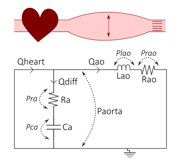
The DAE model is a simple cardiovascular model, where the cardiovascular system is represented by a lumped parameter/0-dimensional model. In the model, the cardiovascular system is represented as an electrical circuit, as seen in the Figure 1.

Figure 1. The example DAE model, where the cardiovascular system with the heart and elastic aorta (top) is represented by an electrical circuit (bottom).
When the equations are derived from the circuit using current and voltage laws such as Kirchhoff's laws, both ODEs and DAEs can emerge. This model file in this example contains both ODEs:
\(d/dt(Pca) = Qdiff/Ca\)
\(d/dt(Qao) = Plao/Lao\)
and DAEs:
\(0 = Qheart - Qdiff - Qao\)
\(0 = Pca + Pra - Prao - Plao\)
The full model file is shown below and can be downloaded here: dae model
########## NAME
dae
########## METADATA
time_unit = s
########## MACROS
########## STATES
// ODEs
d/dt(Pca) = Qdiff/Ca
d/dt(Qao) = Plao/Lao

// DAEs
0 = Qheart - Qdiff - Qao
0 = Pca + Pra - Prao - Plao

// Initial conditions
Pca(0)         = 0
Qao(0)         = 0
Qdiff(0)       = 0
Plao(0)        = 0

########## PARAMETERS
Ca =  1.1
Ra = 0.1
Rao = 1.2
Lao = 0.0005

########## VARIABLES
// Define function for heart beats
k_syst = 0.4
Qheart = ceil(max(0,k_syst-fmod(time,T)/T))  * 300.*sin((CONSTANT_PI*(fmod(time,T)/T))/k_syst)

Pra = Ra*Qdiff
Prao = Rao*Qao

########## FUNCTIONS
########## EVENTS

########## OUTPUTS
########## INPUTS
T = T_in @ 1 // @ 1 means that T has the value 1 if T_in is not given as input

########## FEATURES
Aortic pressure = Pca + Pra [mmHg]

// Extra features to better understand the model:
Flow input Qheart = Qheart [ml/s]
Qdiff = Qdiff  [ml/s]
Qao = Qao   [ml/s]
Pca = Pca  [mmHg]
Plao = Plao  [mmHg]
KCL = Qheart - Qdiff - Qao [ml/s]
KVL = Pca + Pra - Prao - Plao [mmHg]
Simulating the model
A DAE model is simulated in the same way as any other model object in SUND, by installing and importing the model and then creating a simulation object which can be simulated. However, some simulation settings might need to be changed:
Simulation settings
Since it is a DAE model, we need to have consistent initial conditions for all DAEs and ODEs when the simulation starts.
To make sure this is the case, we set the option calc_ic to Truefor the solver to calculate consistent initial conditions for the algebraic states and differential derivatives by using the given initial conditions for the differential states.
The option is called calc_ic, and the default value is False.
# Let the solver calculate consistent initial conditions for all DAEs and ODEs
options = sim.get_options()
print(f'Option calc_ic before change: {options['calc_ic']}')
options['calc_ic'] = True
sim.set_options(options)
print(f'Option calc_ic after change: {options['calc_ic']}')
Simulation
Since the cardiovascular model is oscillating for each heartbeat, it needs to be simulated for a certain amount of time until the oscillations have been stabilized.
In this example, the model is simulated for 20 cardiac cycles (T is the length of one cardiac cycle) to reach the steady state before the actual simulation is done.
# First, we could simulate the model for 20 heartbeats to reach a steady state
sim.simulate(time_vector = np.arange(0, T*20, 0.001),
            reset = True,
            options = options)

# Then, we continue the simulation by simulating the wanted timepoints
# Define timepoints for the simulation
number_of_heartbeats = 2
timepoints = np.arange(0, T*number_of_heartbeats, 0.001)
# Simulate
sim.simulate(time_vector = timepoints,
            reset = False,
            options = options)
Full python code to run the example
The full code to run the example is shown below, but it can also be downloaded here.
Requirements
To run this example code, the following python packages are needed in addition to the SUND package
uv add numpy matplotlib
pip install numpy matplotlib
Example code
import os

import matplotlib.pyplot as plt
import numpy as np

import sund

#%% Print the model to a file called 'dae.txt', located in a folder called modelfiles
os.makedirs('./modelfiles', exist_ok=True)

MODEL_NAME = "dae"

#%% Install and load the model
sund.install_model(f"modelfiles/{MODEL_NAME}.txt")
model = sund.load_model(f"{MODEL_NAME}")

#%%  Create an activity to set cardiac cycle length
T = 0.86 #length of cardiac cycle
activityT = sund.Activity(time_unit='s')
activityT.add_output(sund.PIECEWISE_CONSTANT, "T_in", t = [0], f=[1,T])

#%% Create a simulation object
sim = sund.Simulation(model,activities = activityT, time_unit = 's')

#%% DAE settings
# We set the option for the solver to calculate consistent initial conditions for the  algebraic states
# and differential derivatives by using the given initial conditions for the differential states.
# The option is called 'calc_ic', and the default value is false.
options = sim.get_options()
print(f'Option calc_ic before change: {options['calc_ic']}')
options['calc_ic'] = True
print(f'Option calc_ic after change: {options['calc_ic']}')

# Sometimes, the 'abs_tol' and 'rel_tol' options need to be adjusted to get a good solution.
options['abs_tol'] = 1e-11
options['rel_tol'] = 1e-08

sim.set_options(options)

#%% Run the simulation
# First, we could simulate the model for 20 heartbeats to reach a steady state
sim.simulate(time_vector = np.arange(0, T*20, 0.001),
            reset = True,
            options = options)

# Then, we continue the simulation by simulating the wanted timepoints
# Define timepoints for the simulation
number_of_heartbeats = 2
timepoints = np.arange(0, T*number_of_heartbeats, 0.001)
# Simulate
sim.simulate(time_vector = timepoints,
            reset = False,
            options = options)

#%% Plot the resulting simulation, for example the feature 'Aortic pressure'
feature_to_plot = 'Aortic pressure'
feature_idx = sim.feature_names.index(feature_to_plot)
plt.figure()
plt.plot(sim.time_vector, sim.feature_data[:,feature_idx])
plt.xlabel(f"Time ({sim.time_unit})")
plt.ylabel(f"{feature_to_plot} ({sim.feature_units[feature_idx]})")
plt.show()