Comparision between sund and scipy.odeit
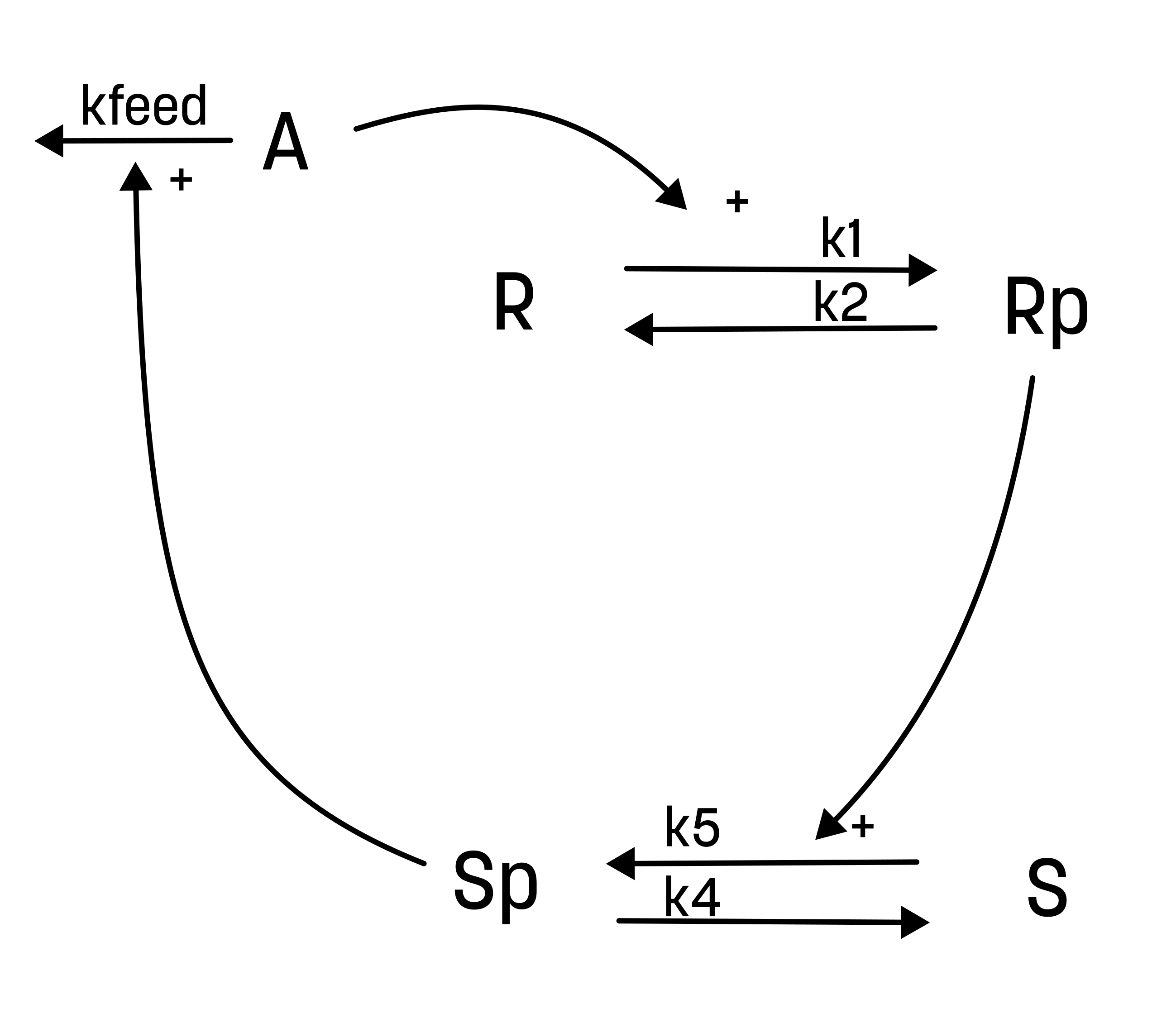
In this example/benchmark, we will simulate the following model, where the value of the input (A) is set to 1 at time points 0 and 2. And we simulate for 5 minutes in total. Furthermore, we will simulate the model with an inhibition, that effectively reduces the rate of k1 to half (i.e. k1_inhibited = k1*0.5), starting from t = 2.
# Import packages
import sund
from scipy.integrate import odeint
import matplotlib.pyplot as plt
import numpy as np
SUND implementation
In this implementation, we use an event to set the value of (A), whenever the input (A_in) is set greater than 0.
First, we need to create the model file. Typically, this is done in a text-editor but here we do it by writing the model to a file. Then, we install and load the model.
# Save the model to file:
sund_model_definition = """\
########## NAME
sund_model

########## METADATA
time_unit = m
########## MACROS
########## STATES
d/dt(R) = r2-r1
d/dt(Rp) = r1-r2
d/dt(S) = r4-r5
d/dt(Sp) = r5-r4
d/dt(A) = - r3

R(0) = 1.0
Rp(0) = 0.0
S(0) = 1.0
Sp(0) = 0.0
A(0) = 0.0

########## PARAMETERS
k1 = 5.0
k2 = 20.0
kfeed = 10.0
k4 = 15.0
k5 = 30.0

########## VARIABLES
r1 = R*A*k1 * (1-inhib)
r2 = Rp*k2
r3 = A*Sp*kfeed
r4 = Sp*k4
r5 = S*Rp*k5

########## FUNCTIONS
########## EVENTS
event1 = A_in>0, A, A_in // When the input A_in is greater than 0, set A to A_in

########## OUTPUTS
########## INPUTS
A_in = A_in @ 0
inhib = inhib @ 0
########## FEATURES
A_in = A_in
inhib = inhib
A = A
R = R
Rp = Rp
S = S
Sp = Sp
"""


# Install and load the model
sund.install_model(sund_model_definition)
model = sund.load_model("sund_model")
Model 'sund_model' succesfully installed.
Now, we need to set up the inputs (with activity objects). Since we set the value of A with the event when A_in>0, we also need to toggle of the input in between the times 0 and 2.
# Define the activity object
activation = sund.Activity(time_unit = 'm')
activation.add_output(name="A_in", type="piecewise_constant", t = [0, 0.5, 2, 2.5], f=[0, 1, 0, 1, 0])

inhibition = sund.Activity(time_unit = 'm')
inhibition.add_output(name="inhib", type="piecewise_constant",t = [2], f=[0, 0.5])
Now, we can set up the simulation and run it.
simulation_sund = sund.Simulation(time_unit = 'm',
                      models = [model],
                      activities = [activation],
                      time_vector = np.linspace(0, 5, 1000)
)
simulation_sund_inhibition = sund.Simulation(time_unit = 'm',
                        models = [model],
                        activities = [activation, inhibition],
                        time_vector = np.linspace(0, 5, 1000)
    )

simulation_sund.simulate()
simulation_sund_inhibition.simulate()
Finally, we plot the features of the model we defined (the input and the states)
# Create the plot
fig, ax = plt.subplots(3, 2, figsize=(10, 8), sharex=True)

for sim_type, sim in zip(["normal", "inhibition"],[simulation_sund, simulation_sund_inhibition]):
    # Get the results as a dictionary
    feature_dict = sim.feature_data_as_dict()

    # Plot the results
    if sim_type == "normal":
        ax[0, 0].plot(sim.time_vector, feature_dict['A_in'], label='A_in', color = 'black')
        ax[0, 0].plot(sim.time_vector, feature_dict['inhib'], label='inhib', color = 'grey')

    ax[0, 1].plot(sim.time_vector, feature_dict['A'], label=sim_type)
    ax[1, 0].plot(sim.time_vector, feature_dict['R'], label=sim_type)
    ax[1, 1].plot(sim.time_vector, feature_dict['Rp'], label=sim_type)
    ax[2, 0].plot(sim.time_vector, feature_dict['S'], label=sim_type)
    ax[2, 1].plot(sim.time_vector, feature_dict['Sp'], label=sim_type)

# Set the titles and labels
ax[0, 0].set_ylabel('Inputs')
ax[0, 0].legend()
ax[0, 1].set_ylabel('A')
ax[0, 1].legend()
ax[1, 0].set_ylabel('R')
ax[1, 0].legend()
ax[1, 1].set_ylabel('Rp')
ax[1, 1].legend()
ax[2, 0].set_ylabel('S')
ax[2, 0].set_xlabel('Time (m)')
ax[2, 0].legend()
ax[2, 1].set_ylabel('Sp')
ax[2, 1].set_xlabel('Time (m)')
ax[2, 1].legend()

fig.suptitle('SUND simulation results')
Text(0.5, 0.98, 'SUND simulation results')

Simulating with SciPy.integrate.odeint
Here, we also want to do two simulation, either with or without the inhibition, and with setting of the input (A) at t=0 and t=2, simulating between 0 and 5.
Since it is not possible to manipulate the values or A directly in the ODE function, we need to subdivide the integration into two steps
First we create the models
# Implement a model of the second hypothesis here
def scipy_model(state,t, param):

    # Define the states
    R = state[0]
    Rp = state[1]
    S = state[2]
    Sp = state[3]
    A = state[4] # A should be the last state in the model for the rest of the code to work properly

    # Define the parameter values
    k1 = param[0]
    k2 = param[1]
    kfeed = param[2]
    k4 = param[3]
    k5 = param[4]

    # Define the reactions
    r1 = R*A*k1
    r2 = Rp*k2
    r3 = A*Sp*kfeed
    r4 = Sp*k4
    r5 = S*Rp*k5

    # Define the ODEs
    ddt_R = -r1+r2
    ddt_Rp = r1-r2
    ddt_S = r4-r5
    ddt_Sp = r5-r4
    ddt_A = -r3

    return[ddt_R, ddt_Rp, ddt_S, ddt_Sp, ddt_A]


def scipy_model_inhib(state,t, param):

    if t>2:
        inhib = 0.5
    else:
        inhib = 0

    # Define the states
    R = state[0]
    Rp = state[1]
    S = state[2]
    Sp = state[3]
    A = state[4] # A should be the last state in the model for the rest of the code to work properly

    # Define the parameter values
    k1 = param[0]
    k2 = param[1]
    kfeed = param[2]
    k4 = param[3]
    k5 = param[4]

    # Define the reactions
    r1 = R*A*k1 * (1-inhib)
    r2 = Rp*k2
    r3 = A*Sp*kfeed
    r4 = Sp*k4
    r5 = S*Rp*k5

    # Define the ODEs
    ddt_R = -r1+r2
    ddt_Rp = r1-r2
    ddt_S = r4-r5
    ddt_Sp = r5-r4
    ddt_A = -r3

    return[ddt_R, ddt_Rp, ddt_S, ddt_Sp, ddt_A]
Next, we run the simulations and plot the results
param = [5, 20, 10, 15, 30] # = [k1, k2, kfeed, k4, k5]
ic = [1, 0, 1, 0, 1] # = [R(0), Rp(0), S(0), Sp(0), A(0)]
time_vector = np.linspace(0, 5, 1000)

# Simulate the normal model stepwise
t1 = np.linspace(0, 2, 500)
t2 = np.linspace(2, 5, 500)

## First simulation
sim1 = odeint(scipy_model, ic, t1, (param,))
ic_1 = sim1[-1] # Use the last state of the first simulation as the initial condition for the second simulation
ic_1[4] = 1 # Set A to 1 for the second simulation

## Second simulation
sim2 = odeint(scipy_model, ic_1, t2, (param,))
# Concatenate the two simulations (but exclude the last point of the first simulation)
simulation_scipy = np.concatenate((sim1[:-1], sim2), axis=0)
time_vector = np.concatenate((t1[:-1], t2), axis=0)


# Simulate the inhibition model stepwise
sim1_inhib = odeint(scipy_model_inhib, ic, t1, (param,))
ic_inhib_1 = sim1_inhib[-1] # Use the last state of the first simulation as the initial condition for the second simulation
ic_inhib_1[4] = 1 # Set A to 1 for the second simulation

## Second simulation
sim2_inhib = odeint(scipy_model_inhib, ic_inhib_1, t2, (param,))
# Concatenate the two simulations (but exclude the last point of the first simulation)
simulation_scipy_inhib = np.concatenate((sim1_inhib[:-1], sim2_inhib), axis=0)

# Plot the results
fig, ax = plt.subplots(3, 2, figsize=(10, 8), sharex=True)

for sim_type, sim in zip(["normal", "inhibition"],[simulation_scipy, simulation_scipy_inhib]):
    ax[0, 1].plot(time_vector, sim[:, 4], label=sim_type)
    ax[1, 0].plot(time_vector, sim[:, 0], label=sim_type)
    ax[1, 1].plot(time_vector, sim[:, 1], label=sim_type)
    ax[2, 0].plot(time_vector, sim[:, 2], label=sim_type)
    ax[2, 1].plot(time_vector, sim[:, 3], label=sim_type)

# Set the titles and labels
ax[0, 1].set_ylabel('A')
ax[0, 1].legend()
ax[1, 0].set_ylabel('R')
ax[1, 0].legend()
ax[1, 1].set_ylabel('Rp')
ax[1, 1].legend()
ax[2, 0].set_ylabel('S')
ax[2, 0].set_xlabel('Time (m)')
ax[2, 0].legend()
ax[2, 1].set_ylabel('Sp')
ax[2, 1].set_xlabel('Time (m)')
ax[2, 1].legend()

fig.suptitle('Scipy simulation results')

plt.show()

Comparing the SUND simulations with the SciPy odeint simulations
Now, let's compare the simulation from SUND (solid lines) with the simulations from SciPy odeint (dashed lines).
As can be seen, the two methods overlap fully.
# Create the figure
fig, ax = plt.subplots(3, 2, figsize=(10, 8), sharex=True)

# Plot the SUND results

# Define a list of colorblind-friendly colors
colors = [['#ffc20a', '#0c7BDC'], ['#e66100', '#5d3a9b']] # Colorblind-friendly colors

for color, sim_type, sim_sund, sim_scipy in zip(colors, ["normal", "inhibition"],[simulation_sund, simulation_sund_inhibition], [simulation_scipy, simulation_scipy_inhib]):
    # Get the results as a dictionary
    feature_dict = sim_sund.feature_data_as_dict()

    # Plot the SUND results
    ax[0, 1].plot(sim_sund.time_vector, feature_dict['A'], label=f'{sim_type}-SUND', linewidth=2, color=color[0])
    ax[1, 0].plot(sim_sund.time_vector, feature_dict['R'], label=f'{sim_type}-SUND', linewidth=2, color=color[0])
    ax[1, 1].plot(sim_sund.time_vector, feature_dict['Rp'], label=f'{sim_type}-SUND', linewidth=2, color=color[0])
    ax[2, 0].plot(sim_sund.time_vector, feature_dict['S'], label=f'{sim_type}-SUND', linewidth=2, color=color[0])
    ax[2, 1].plot(sim_sund.time_vector, feature_dict['Sp'], label=f'{sim_type}-SUND', linewidth=2, color=color[0])

    # Plot he scipy results
    ax[0, 1].plot(time_vector, sim_scipy[:, 4], linestyle=(0, (3, 5)), label=f'{sim_type}-odeint', linewidth=2, color=color[1])
    ax[1, 0].plot(time_vector, sim_scipy[:, 0], linestyle=(0, (3, 5)), label=f'{sim_type}-odeint', linewidth=2, color=color[1])
    ax[1, 1].plot(time_vector, sim_scipy[:, 1], linestyle=(0, (3, 5)), label=f'{sim_type}-odeint', linewidth=2, color=color[1])
    ax[2, 0].plot(time_vector, sim_scipy[:, 2], linestyle=(0, (3, 5)), label=f'{sim_type}-odeint', linewidth=2, color=color[1])
    ax[2, 1].plot(time_vector, sim_scipy[:, 3], linestyle=(0, (3, 5)), label=f'{sim_type}-odeint', linewidth=2, color=color[1])


# Set the titles and labels
ax[0, 1].set_ylabel('A')
ax[0, 1].legend()
ax[1, 0].set_ylabel('R')
ax[1, 0].legend()
ax[1, 1].set_ylabel('Rp')
ax[1, 1].legend()
ax[2, 0].set_ylabel('S')
ax[2, 0].set_xlabel('Time (m)')
ax[2, 0].legend()
ax[2, 1].set_ylabel('Sp')
ax[2, 1].set_xlabel('Time (m)')
ax[2, 1].legend()

# remove the unused first subplot
ax[0, 0].axis('off')

fig.suptitle('SUND vs. Scipy simulation results')

plt.show()
