A minimal model trained on synthetic data
This example will cover most steps of a systems biology problem on a small model and synthetic data. It will:
- Implement and simulate the model,
- evaluate a start guess of the parameter values,
- improve the values using optimization,
- gather the model uncertainty,
- predict a new experiment,
- and finally compare it to experimental data.
This section refers to an implementation of a model used in a computer exercise. We assume that the model below is saved in a file named M1.txt
The model
########## NAME
M1
########## METADATA
time_unit = m
########## MACROS
########## STATES
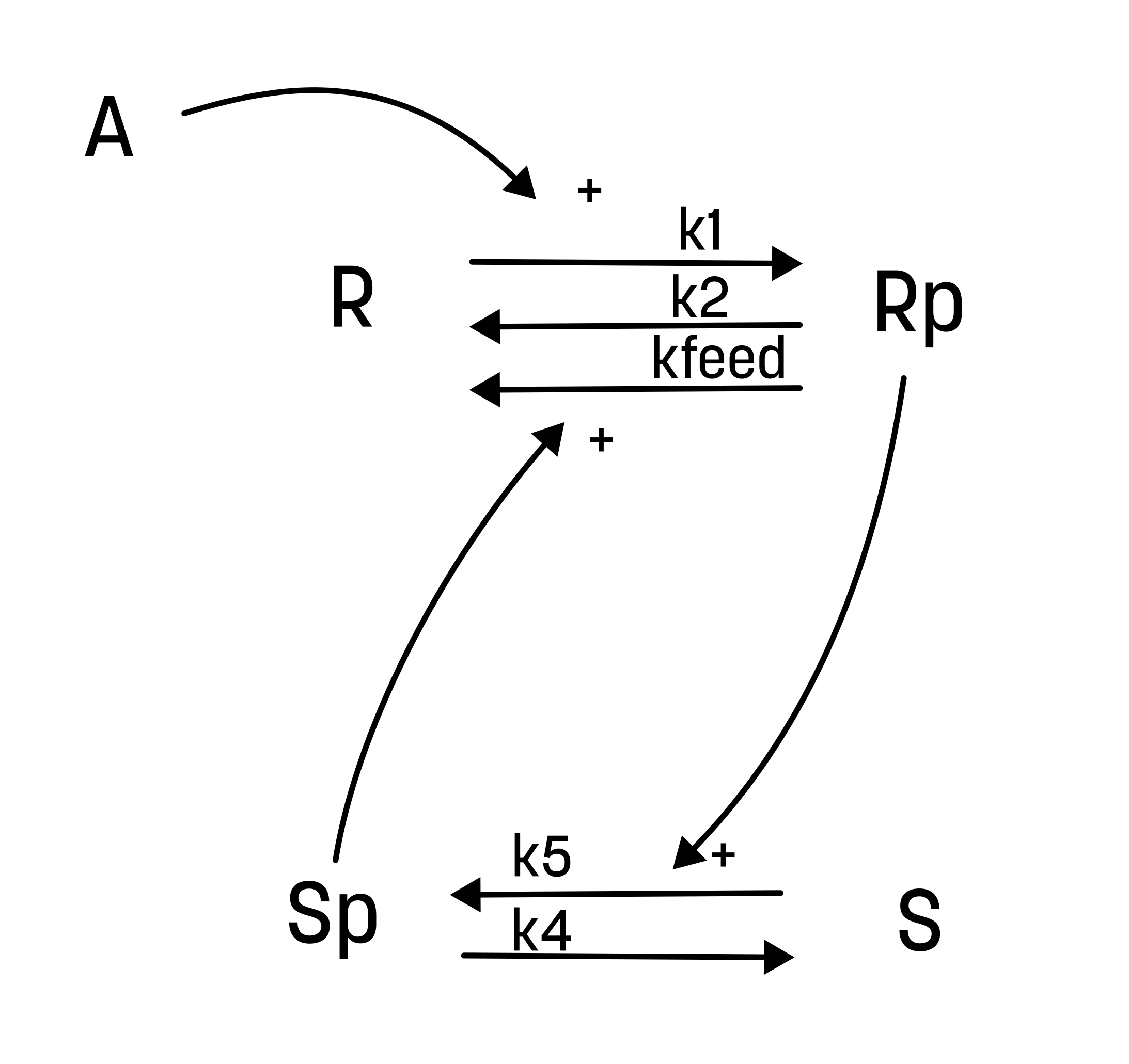
d/dt(R) = r3+r2-r1
d/dt(Rp) = r1-r2-r3
d/dt(S) = r4-r5
d/dt(Sp) = r5-r4
R(0) = 1.0
Rp(0) = 0.0
S(0) = 1.0
Sp(0) = 0.0
########## PARAMETERS
k1 = 1.0
k2 = 0.0001
kfeed = 1000000.0
k4 = 1.0
k5 = 0.001
########## VARIABLES
r1 = R*A*k1
r2 = Rp*k2
r3 = Rp*Sp*kfeed
r4 = Sp*k4
r5 = S*Rp*k5
########## FUNCTIONS
########## EVENTS
########## OUTPUTS
########## INPUTS
A = activation @ 1
########## FEATURES
EGFRp = Rp
The Python code
Before you start, you should download the experimental dataset (right-click and save) and the model file. The code is given below, but you can also download the file from here.
Required packages
For this code to work, you need some packages (in addition to the SUND package). Install them with
uv add numpy scipy matplotlib
pip install numpy scipy matplotlib
The full Python code
#%% Import packages
import csv
import json
import random
from pathlib import Path

import matplotlib.pyplot as plt
import numpy as np
from scipy.optimize import Bounds, differential_evolution
from scipy.stats import chi2

import sund

# Create a numpy serializer for json
class NumpyEncoder(json.JSONEncoder):
    def default(self, obj):
        if isinstance(obj, np.ndarray):
            return obj.tolist()
        return super().default(obj)

#%% Load and print the data
data = json.loads(Path("data_2025-05-22.json").read_text())


for experiment in data:
    all_times = [t for observable in data[experiment]["observables"]
                 for t in data[experiment]["observables"][observable]["time"]]
    data[experiment]["all_times"] = sorted([float(x) for x in np.unique(all_times)])  # Store the time vector for each experiment


# split the data into training and validation data
data_validation = {}
data_validation['step_dose'] = data.pop('step_dose')

print(data)

#%% Plot the data
def plot_dataset(data, FC='k'):
    plt.errorbar(data['time'], data['mean'], data['SEM'], linestyle='None', marker='o', markerfacecolor=FC, color='k', capsize=5)
    plt.xlabel('Time (minutes)')
    plt.ylabel('Phosphorylation (a.u.)')

# Define a function to plot all datasets
def plot_data(data):
  for idx, experiment in enumerate(data):

        for observable_name, observable_data in data[experiment]["observables"].items():
            plt.figure(idx)
            plot_dataset(observable_data)
            plt.title(f'EGFR - {experiment}')

plot_data(data)

#%% Install the model
sund.install_model('M1.txt')
print(sund.installed_models())

#%% Load the model object
m1 = sund.load_model("M1")

#%% Create a activity objects
activity1 = sund.Activity(time_unit='m')
activity1.add_output(type="piecewise_constant", name="activation", t = data['dose1']['inputs']['activation']['t'], f=data['dose1']['inputs']['activation']['f'])

activity2 = sund.Activity(time_unit='m')
activity2.add_output(type="piecewise_constant", name="activation", t = data['dose2']['inputs']['activation']['t'], f=data['dose2']['inputs']['activation']['f'])

#%% Create simulation objects
m1_sims = {}
m1_sims['dose1'] = sund.Simulation(models = m1, activities = activity1, time_unit = 'm', time_vector = data['dose1']['all_times'])
m1_sims['dose2'] = sund.Simulation(models = m1, activities = activity2, time_unit = 'm', time_vector = data['dose2']['all_times'])

#%% Define two function to plot the model simulation and data
def plot_simulation(params, sim, timepoints, color='b', feature_to_plot='EGFRp'):
    # Setup, simulate, and plot the model
    sim.simulate(time_vector = timepoints,
                    parameter_values = params,
                    reset = True)

    feature_idx = sim.feature_names.index(feature_to_plot)
    plt.plot(sim.time_vector, sim.feature_data[:,feature_idx], color)

def plot_sim_with_data(params, sims, data, color='b'):
    for idx, experiment in enumerate(data):
        for observable_name, observable_data in data[experiment]["observables"].items():
            plt.figure()
            timepoints = np.arange(0, data[experiment]["all_times"][-1]+0.01, 0.01)
            plot_simulation(params, sims[experiment], timepoints, color)
            plot_dataset(observable_data)
            plt.title(f'EGFR - {experiment}')

#%% Plot the simulation given the initial parameter values, along with the data
params0_M1 = [1, 0.0001, 1000000, 1, 0.001] # = [k1, k2, kfeed, k4, k5]
plot_sim_with_data(params0_M1, m1_sims, data)

#%%  Define a function to calculate the cost
def fcost(params, sims, data):
    cost=0
    for experiment, dataset in data.items():
        try:
            sims[experiment].simulate(
                time_vector = dataset["all_times"],
                parameter_values = params,
                reset = True)

            for observable_key, observable_data in dataset["observables"].items():
                y_sim = sims[experiment].feature_data[:,0]
                y = observable_data["mean"]
                SEM = observable_data["SEM"]

                cost += np.sum(np.square(((y_sim - y) / SEM)))

        except Exception as e:
            if "CVODE" not in str(e):
                raise e

            cost+=1e30  # in-case of exception add a "high cost"

    return cost

#%% Improving the agreement manually
param_guess_M1 = [1, 0.0001, 1000000, 1, 0.01] # Change the values here and try to find a better agreement

cost =  fcost(param_guess_M1, m1_sims, data)
print(f"Cost of the M1 model: {cost}")

dgf=0
for experiment in data:
    for observable in data[experiment]["observables"]:
        dgf += np.count_nonzero(np.isfinite(data[experiment]["observables"][observable]["SEM"]))
chi2_limit = chi2.ppf(0.95, dgf)
print(f"Chi2 limit: {chi2_limit}")
print(f"Cost > limit (rejected?): {cost>chi2_limit}")

plot_sim_with_data(param_guess_M1, m1_sims, data)

#%% Improving the agreement using optimization methods
def callback_M1(x,convergence):
    out = {"x": list(x)}
    Path("M1-temp.json").write_text(json.dumps(out, cls=NumpyEncoder))

args_M1 = (m1_sims, data)

#%% Convert to log scale
x0_log_M1 = np.log(param_guess_M1)
bounds_M1_log = Bounds([np.log(1e-6)]*len(x0_log_M1), [np.log(1e6)]*len(x0_log_M1)) # Create a bounds object needed for some of the solvers

def fcost_log(params_log, sim, data):
    params = np.exp(params_log.copy())
    return fcost(params, sim, data)

def callback_M1_log(x,convergence):
    callback_M1(np.exp(x.copy()),convergence)

res = differential_evolution(func=fcost_log, bounds=bounds_M1_log, args=args_M1, x0=x0_log_M1, callback=callback_M1_log, disp=True) # This is the optimization
res['x'] = np.exp(res['x']) # convert back from log scale

print(f"\nOptimized parameter values: {res['x']}")
print(f"Optimized cost: {res['fun']}")
print(f"chi2-limit: {chi2_limit}")
print(f"Cost > limit (rejected?): {res['fun']>chi2_limit}")

if res['fun'] < chi2_limit: #Saves the parameter values, if the cost was below the limit.
    file_name = f"M1 ({res['fun']:.3f}).json"
    res_out = {"f": res["fun"], "x": list(res["x"])}
    Path(file_name).write_text(json.dumps(res_out, cls=NumpyEncoder))

#%% Plot the simulation given the optimized parameters
p_opt_M1 = res['x']
plot_sim_with_data(p_opt_M1, m1_sims, data)

#%% Setup for saving acceptable parameters
all_params_M1 = [] # Initiate an empty list to store all parameters that are below the chi2 limit

def fcost_uncertainty_M1(param_log, model, data):

    param = np.exp(param_log) # Assumes we are searching in log-space
    cost = fcost(param, model, data) # Calculate the cost using fcost

    # Save the parameter set if the cost is below the limit
    if cost < chi2.ppf(0.95, dgf):
        all_params_M1.append(param)
    return cost

#%% Run the optimization a few times to save some parameters
for i in range(0,5):
    res = differential_evolution(func=fcost_uncertainty_M1, bounds=bounds_M1_log, args=args_M1, x0=x0_log_M1, callback=callback_M1_log, disp=True) # This is the optimization
    x0_log_M1 = res['x']
print(f"Number of parameter sets collected: {len(all_params_M1)}") # Prints now many parameter sets that were accepted

#%% Save the accepted parameters to a csv file
with Path('all_params_M1.csv').open('w', newline='') as csvfile:
    writer = csv.writer(csvfile, delimiter=',')
    writer.writerows(all_params_M1)

#%% Plot model uncertainty
# Define a function to plot the model uncertainty
def plot_uncertainty(all_params, sims, data, c='b', n_params_to_plot=500):
    random.shuffle(all_params)

    for idx, experiment in enumerate(data):
        # Plot the simulations
        for observable_name, observable_data in data[experiment]["observables"].items():
            plt.figure(idx) # Create a new figure
            timepoints = np.arange(0, data[experiment]["all_times"][-1]+0.01, 0.01)

            for param in all_params[:n_params_to_plot]:
                plot_simulation(param, sims[experiment], timepoints, c)

            # Plot the data
            if "step_dose" in experiment:
                color = 'w'
            else:
                color = 'k'
            plot_dataset(observable_data, color)

            plt.title(f'EGFR - {experiment}')

# Plot the uncertainty for the model
plot_uncertainty(all_params_M1, m1_sims, data)

#%% Setup for simulating the new prediction

m1_pred_sims = {}
for key, value in data_validation.items():
    act_prediction = sund.Activity(time_unit='m')
    act_prediction.add_output(
        name = "activation",
        type = "piecewise_constant",
        t=value["inputs"]["activation"]["t"],
        f = value["inputs"]["activation"]["f"])

    m1_pred_sims[key] = sund.Simulation(models = m1, time_unit = 'm', activities = act_prediction)

#%% Plot model predict with the experimental data
plot_uncertainty(all_params_M1, m1_pred_sims, data_validation)


# show all the plots
plt.tight_layout()
plt.savefig("model prediction_example.png", dpi=300)
plt.show()